 Methodology
This methodology was originally written in October 2026. While we plan to maintain and update this explorer over time, the examples here reflect the estimates and robustness checks carried out on the most recent data at the time the explorer was created.
1. How we estimate chip arrivals
This dataset estimates how much AI compute arrives in each country, by quarter, from 2022 to the present, in H100-equivalents (H100e), chip units, and trade value. It relies primarily on customs records, except for Chinese domestic production, where we use estimates from our AI chip sales explorer.
Almost all advanced AI chips are fabricated in Taiwan. While some advanced logic dies are now manufactured in the US, and the most valuable component, memory, comes primarily from South Korea, these components undergo advanced packaging to turn into a GPU or other advanced AI accelerator predominantly in Taiwan. Then, most of these AI chips cross at least one border between their creation in Taiwan and the data center where they run, often undergoing additional packaging and assembly between departing Taiwan and arriving at their final destination.
Most countries publish monthly records of what crosses their borders, by product code, partner country, piece count, and value. The product codes we track contain both AI and non-AI chips, as well as chips and non-chip components, so we need to estimate the share of AI chips. We also need to account for some chips crossing multiple borders between leaving Taiwan and entering the country where they are installed and used.
What data we use
We collect monthly customs data for 16 destinations with their own records: the US, China, Hong Kong, the EU (as one bloc), South Korea, Malaysia, Singapore, the UK, Japan, Indonesia, India, Thailand and Mexico, plus Saudi Arabia, Australia and Canada through UN Comtrade. We also use Taiwan’s export records. We count four server and parts codes (8471.49, complete systems; 8471.50, servers; 8471.80, other computer units; and 8473.30, parts, including boards and cards), using 2021 as a baseline year, and supplement our analysis with other products and more detailed country-specific codes.
Four steps from customs records to chips by country
- Hardware retained in each country. We count hardware only in the country where it stays, subtracting re-exports and the imported content of servers a country assembles and ships on (Section 3.2).
- AI-related trade. We estimate AI-related trade as the excess above a baseline built from each country’s 2021 trade (Section 3.3).
- Accelerator share of trade value. We estimate how much of the remaining value is the AI chip itself, rather than CPUs, memory, networking or chassis, using national tariff descriptions, and declared value per unit and per kilogram (Section 3.4).
- Allocation of chips to countries. We split our chip sales estimates, by chip model and quarter, across countries in proportion to their chip dollars, assuming chips arrive about two months after they are sold. Huawei and Cambricon chips, which never cross a border, go to China. China’s dollars for diverted chips are adjusted for the premium paid above list price (Sections 4.1–4.3).
Countries whose customs data we do not collect directly, mostly those with a small share of chip trade or those that do not publish their own customs data, are estimated from what other countries declare shipping to them.
How well the estimates match chip sales
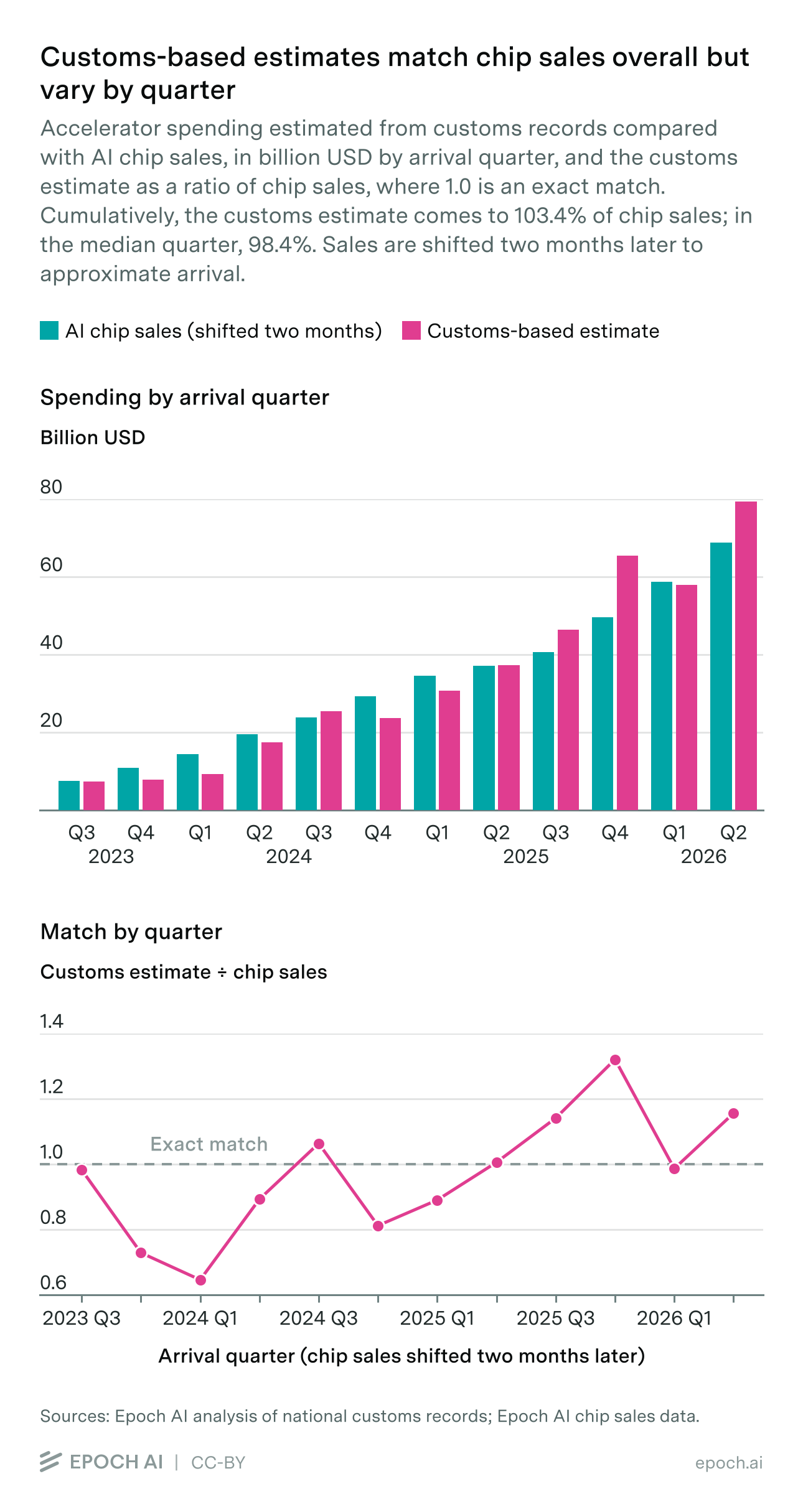
As a check, customs-derived chip spending over arrival quarters 2023Q3–2026Q2 comes to 103.4% of the value of the corresponding chips in our sales data; individual quarters differ by 14.6% on average (see the comparison with chip sales). The check isn’t fully independent, because estimating chip content uses our chip prices and product mix.
Allocating the model-level quantities from chip sales using customs geography gives an estimated 27 million H100-equivalents of cumulative arrivals through June 2026. This includes sales recorded since the start of 2022, with an assumed two-month delay before arrival. Some of these chips might not be operational yet, and some chips may be in transit in one country before being shipped to their end use location.
| Country | Primary estimate, M H100e | Share |
|---|---|---|
| United States | 19.764 | 72.16% |
| China | 2.637 | 9.63% |
| European Union | 1.388 | 5.07% |
| Malaysia | 0.668 | 2.44% |
| India | 0.442 | 1.61% |
| Japan | 0.432 | 1.58% |
| Australia | 0.386 | 1.41% |
| United Kingdom | 0.340 | 1.24% |
| Indonesia | 0.219 | 0.80% |
| South Korea | 0.105 | 0.38% |
| All others | 1.009 | 3.68% |
As of 2026Q2, the US has received 66.8% of allocated AI chips and 72.2% of H100-equivalent compute; China received 18.2% of units and 9.6% of compute. These differences depend on model eligibility and the assumed model mix within each eligible group.
How sensitive the results are
The US is robustly the destination of the majority of the compute across the tested modelling assumptions. China, the EU and several smaller destinations are more sensitive to how we distinguish ordinary trade from accelerator shipments. Their structural ranges are substantially wider than intervals obtained by varying parameters within the adopted model (see Section 4.5).
The data also catches some hardware being routed around export controls, as described in this piece on chip smuggling via Malaysia.
The rest of this methodology covers:
- The trade data (Section 2): product codes, sources, publication schedules and data limitations.
- Methodology (Section 3): each step from customs values to chip dollars, and the comparison with chip sales.
- Country estimates (Section 4): allocating chips and compute to countries, and uncertainty.
- Data quality checks (Section 5): how countries’ records of the same trade compare, a closer look at Taiwan, and why we use national records rather than BACI’s reconciled estimates.
- Robustness checks: at every step we report the variants we tested and the known weaknesses of each.
Note: parts of the sections below were drafted with AI assistance.
2. The customs data we use
2.1 Why we use customs data
Goods are classified using Harmonised System (HS) commodity codes. The first six digits identify an internationally standardized category; countries can add digits to distinguish more specific products. For example, 847330 covers computer parts and accessories, while Japan’s nine-digit import code 847330011 identifies DRAM modules within that category.
Four properties make customs data attractive:
- It has broad coverage. Customs statistics come from declarations required for international shipments, giving them broad coverage without relying on a voluntary survey. Coverage and accuracy nevertheless vary: records can contain missing shipments, incorrect classifications, valuation errors and other reporting problems, including in countries with strong customs enforcement.
- It is high frequency. Taiwan publishes month M about 7–10 days after it ends; Korea, Malaysia, Singapore and Thailand within 3–4 weeks; the US at ~5–6 weeks; the EU’s detailed 8-digit data at ~2 months.
- It is bilateral. Every record has a partner country, so flows are directional and traceable: Taiwan’s exports to Malaysia are a different observation from Malaysia’s imports from Taiwan, which can help us identify discrepancies. Importers’ declarations are also generally more reliable because of tariff and tax implications, while the same incentives do not exist for exports.
- It is granular. National tariff schedules extend the six-digit Harmonised System codes and sometimes isolate useful products. Japan, Korea and the US identify memory modules that can be excluded from accelerator content. Korea’s multichip-memory line also helps trace HBM-related trade with Taiwan, although the code encompasses more than HBM. Product definitions and the limits of these proxies are listed in Section 3.4 and Appendix B.
The main limitation of customs data is that there is no “AI accelerator” code. The last meaningful revision of the HS was done in 2022, before the AI boom. This means that GPUs, AI servers, gaming graphics cards and ordinary rack servers share codes; a GB300 rack and a point-of-sale terminal can both be “automatic data processing units.” Extracting an AI signal therefore requires (a) picking a code basket where AI dominates the recent growth, and (b) explicitly modelling the non-AI part of the flow to remove from said basket.
2.2 Why we do not rely on UN Comtrade alone
UN Comtrade brings together countries’ official trade submissions in a common database, making it a convenient starting point for international comparisons. We use it for additional country coverage and cross-checks, but it alone does not provide the granularity, timeliness or Taiwan coverage this project needs:
- Granularity. Comtrade trims everything to HS-6. The national subdivisions that might isolate HBM, switch/router lines, or GPU add-in cards get discarded.
- Timeliness. Comtrade ingests national submissions and lags them by months, or sometimes over a year. There are also some other quirks: for example, China’s monthly submissions stop at 2024-12, and Thailand is simply missing 2025-03 → 2025-12.
- Coverage. Taiwan does not report to UN Comtrade at all (since it is not a member country). Its national portal is the only source.
Comtrade supplies partner coverage where national extracts are narrow, physical fields where available, and a cross-check on collection. Saudi Arabia, Australia and Canada enter the estimator through their own Comtrade submissions. We also use Comtrade to extend the historical records needed for the 2021 reference and netting warm-up. Taiwan’s history comes from its national portal, while the EU’s comes from Eurostat. The reconstruction of the UK’s 2021 EU imports is described in Section 3.3. For Mexico, the estimator uses INEGI trade values; supplementary INEGI quantities and weights support the sensitivity analysis in Section 3.2.
2.3 How customs records are structured
The unit of observation is a (reporter, flow, partner, commodity code, month) cell with a value in USD (sometimes converted from local currency using IMF data), and, where the source publishes it, a quantity and a net weight. “Reporter” is the country whose customs agency filed the record; “flow” is the direction (import, export, and, in some cases, domestic export vs re-export); “partner” is the other country. This means that every cell should be recorded twice, once by each side of the border, under each side’s own conventions.
2.4 Which product codes we track
Countries report their trade following the Harmonized System. The HS is maintained by the World Customs Organization and used by more than 200 countries covering ~98% of world merchandise trade. It standardizes commodity classification up to six digits and is revised every ~5 years, with the last revision in 2022.
We identify candidate codes from their product descriptions and national tariff subdivisions, then check where the observed accelerator supply-chain growth appears and whether classification differences reconcile across the broader family. The core basket combines processing units, complete computer systems, other computer units and parts. These codes contain both AI and non-AI equipment. We first estimate and subtract a baseline for ordinary computing and component trade. We then estimate how much of the remaining value belongs to accelerator modules, using national product descriptions and declared value per unit or kilogram. The rest can include host memory, CPUs, storage and other system components.
We divide the codes below into two tiers. Tier 1 contains the server, system and parts codes used to estimate accelerator trade and allocate it across countries. Tier 2 covers chips, memory, networking and storage; these codes are used only for diagnostics and supporting analyses, not for the allocation itself. The repository’s code definitions list the codes used by the estimator and explain why bare chips are excluded from the allocation.
Tier 1
| HS-6 | What it is | Why it matters |
|---|---|---|
| 8471.50 | ADP processing units: assembled servers, HGX/DGX boards | The AI-server code. US imports: $37.0B (2023) → $163.7B (2025), and $25.8B in May 2026 alone. |
| 8473.30 | Parts and accessories of ADP machines | GPU cards and boards; second-largest AI flow. |
| 8471.80 | Other ADP units | Small in most countries, but half of Taiwan’s basket exports land here. |
| 8471.49 | ADP systems entered as such | Complete racks entered as one unit. |
Tier 2
Chips, memory, networking and storage: 8542.31 (processors/controllers, i.e. bare accelerator dies), 8542.32 (memory ICs), 8542.39 (other ICs), 8517.62 (switches), 8523.51 (SSDs).
- Bare GPU dies are not where the value is. In US 10-digit data, the dedicated “GPU” chip line is ~3% of HS 8542.31. Accelerator value crosses borders as assembled boards and servers, under 8471.50 and 8473.30.
- The AI signal dominates much of the recent growth, but these codes carry a large pre-existing non-AI business: ordinary servers, consumer graphics cards and PCs. The estimate subtracts a measured non-AI baseline, as described in Section 3.3.
National tariff subdivisions are collected alongside HS-6, and product-code research is part of onboarding each country. Useful distinctions include memory modules, Korean multichip memory and Taiwan’s finished-DRAM line, switching equipment, and sound/video cards. These labels identify different product scopes rather than a common AI-only category. Taiwan’s collected 847150, 847330 and 854231 export trees do not provide a dedicated AI/GPU subdivision. Section 3.4 describes the module exclusions and Appendix B lists the memory diagnostics.
2.5 The countries in the study
We have built fourteen national datasets so far, and three more on UN Comtrade. “Flows” uses the schema’s codes (M import, X total export, DX domestic export, RX re-export); “quantity” and “net weight” show the share of value that has that data.
| Source and access | Flows | Quantity/piece counts | Net weight | Publication lag | |
|---|---|---|---|---|---|
| United States | Census Bureau API, free key, fully automated | M, X, DX, RX | 100% | Only gross weight | ~5–6 wks |
| Taiwan | MOF portal, manual (CAPTCHA) | M, X | 36% | 100% | ~7–10 days |
| China | GACC, manual (slider CAPTCHA on every query) | M, X | 91% | 100% | ~3–4 wks |
| Mexico | INEGI BCMM OLAP cube (9 corridor partners) plus paired Comtrade dataset for all-partner breadth | M, X | National-source counts used in sensitivity tests | M+1 headline, M+3 revised | |
| South Korea | KCS, keyless, automated | M, X | 99.8% | ~M+1, mid-month | |
| Hong Kong | C&SD Trade-IDDS REST API, keyless, automated | M, X, DX, RX | 100% | ~6 wks | |
| Singapore | SingStat TableBuilder API, keyless, automated | M, X, DX, RX | 100% | ~3.5 wks | |
| Malaysia | DOSM METS Online, undocumented JSON API, automated | M, X, DX, RX | 100% (Comtrade submission) | Boards only (Comtrade submission) | ~3 wks |
| Thailand | MOC, documented keyless API | M, X | kg on 100% of imports (11-digit lines) | ~M+1, after the 20th | |
| EU (27 members plus aggregate) | Eurostat COMEXT DS-045409 JSON-stat, keyless, automated | M, X | 28% | 100% | ~M+2, ~15th |
| Japan | e-Stat Trade Statistics, keyless file route, automated | M, X | 96% | 6% | ~M+1 provisional |
| United Kingdom | HMRC uktradeinfo OTS OData, keyless, automated | M, X | 38% | 100% | ~6 wks |
| India | TRADESTAT, keyless web app, automated | M, X | 100% on the machine codes | ~5–6 wks | |
| Indonesia | BPS WebAPI, free personal key, automated | M, X | 100% | ~4–6 wks | |
| Saudi Arabia | UN Comtrade (GASTAT submission), shared puller | M, X | 57% | 100% | ~4–6 months |
| Australia | UN Comtrade (ABS submission), shared puller | M, X | 88% | None | ~2–3 months |
| Canada | UN Comtrade (Statistics Canada submission), shared puller | M, X, DX, RX | 82% | None | ~2–3 months |
The estimator uses import records for sixteen destinations, treating the EU as one bloc. Other destinations are estimated from selected exporters’ declarations. The main collection covers 2022 onwards, supplemented with 2021 trade and reference-index history to establish the baseline and initialize netting. Taiwan’s 2021 exports cover all four counted hardware codes. The historical extension supports the reference calculation; it does not provide the same national-code and physical-field detail as every current dataset. Partner coverage varies by source: Mexico’s monthly national extract covers nine corridors plus a World control. Each source has a standardized dataset and validation checks. Twelve of the fourteen national collection workflows are automated; Taiwan and China require manual downloads.
Coverage gaps include Vietnam, where tariff-line data would require a third-party source, and the UAE, which publishes no usable customs detail and sends no monthly data to Comtrade. Australia, Saudi Arabia and Canada are covered through their HS-6 Comtrade submissions. The same approach could provide destination customs records for Norway, Switzerland, Israel and Brazil.
The data guide lists the sources and required inputs. Each source module documents its publication, code coverage, flows, file formats and treatment of revisions; see, for example, the United States and Taiwan modules.
2.6 How to read customs records
These are properties of customs data that change how the numbers should be read:
-
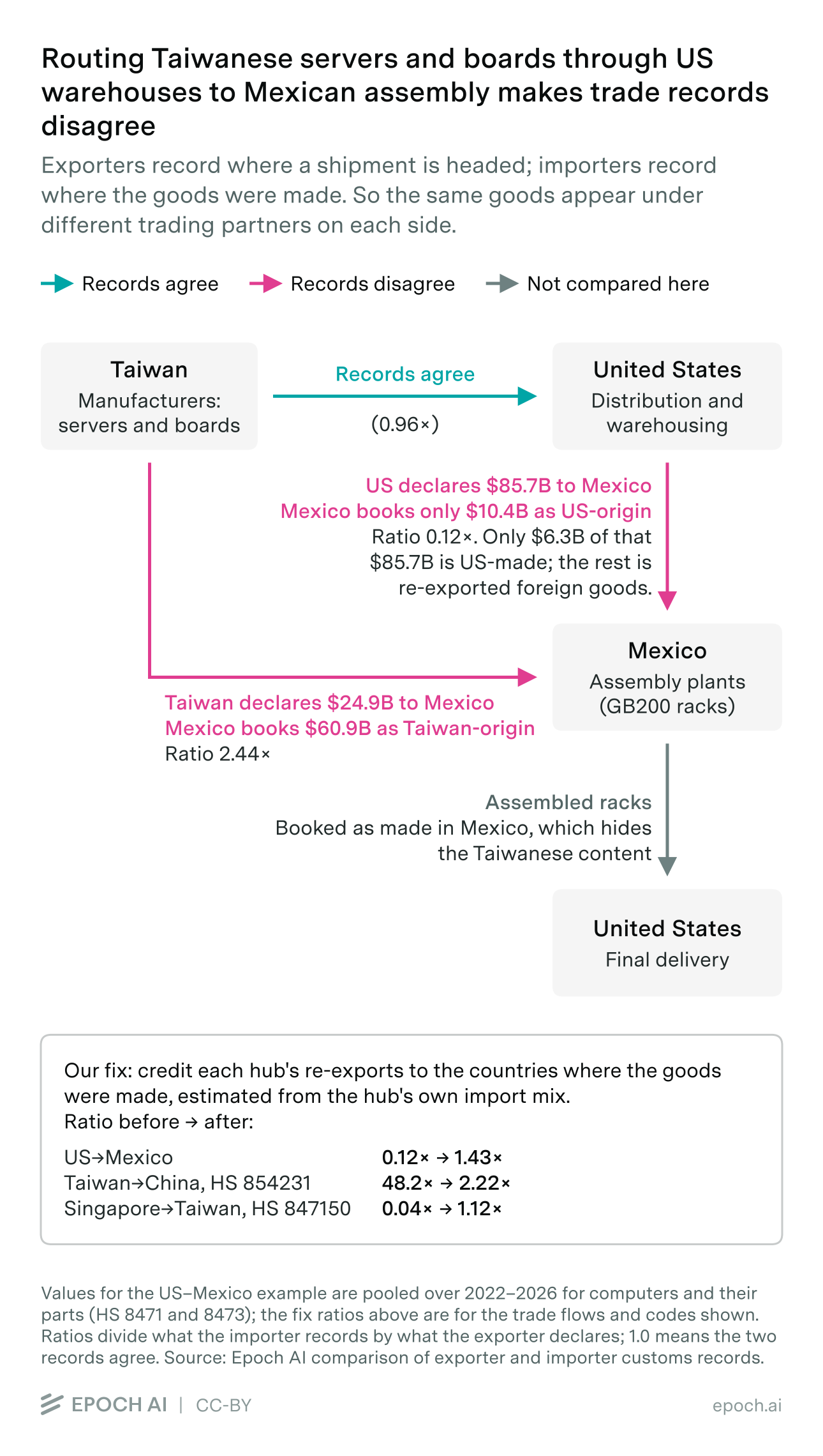
Imports are generally attributed to origin, while exports are attributed to the destination known when the declaration is filed. These need not describe the same leg of a shipment. An exporter may name an intermediary hub or a destination beyond it, while the importing country records where the goods were made. Assembly can change origin; distribution or repackaging generally does not.
For example, the US reports $85.7 billion of server exports to Mexico, while Mexico books only $10.4 billion of arrivals from the US, and books $60.9 billion as Taiwan-origin, more than double the $24.9 billion Taiwan itself reports sending to Mexico. These are Taiwan-built servers passing through US warehouses: the US sees a shipment heading to Mexico and records an export there, Mexico sees Taiwan-made hardware arriving and records an import from Taiwan, and Taiwan sees goods leaving for the US. The two systems record different partner concepts: immediate destination on the export side and country of origin on the import side. Their disagreement therefore does not, by itself, indicate a reporting error.
-
The same goods can be filed under different codes. Taiwan and the US show this most clearly. Compare them code by code and the two sides disagree wildly, anywhere from 0.18× to 2.90× on individual lines. Add the whole 8471 and 8473 family together and they agree to within about 4%: $295.7 billion against $283.2 billion. The two authorities simply sort the hardware into different boxes. Family-level comparisons can reduce discrepancies caused by different commodity classifications.
-
Imports and exports are priced differently. An import value usually includes the freight and insurance (Cost, Insurance, and Freight or CIF) needed to get the goods to the border, while an export value usually stops at the port of departure (Free On Board or FOB). So for the same shipment, the importing country’s figure should come out a little higher than the exporting country’s. Converting records reported in local currency to dollars also introduces exchange-rate noise.
This turns out to explain very little of the disagreement we actually see. Take the corridors where the two sides disagree on value and which also report weight: in 89% of them, the two sides disagree on the tonnage as well. If two countries cannot agree on how many kilograms crossed the border, the gap is not about how the same goods were priced; it is about which goods got counted at all. That leaves freight and insurance able to explain at most about a tenth of the flagged corridors. We still put every country’s import values on the export basis before comparing anything. The US publishes both values for every line, so we measure the freight and insurance margin there, as a curve that falls as goods get more valuable per kilogram, and divide it out of the other countries’ import values. For this hardware the margin is 0.5–1.6% of value (Section 3.2).
-
Recent customs observations can be revised as filings arrive. We exclude incomplete customs quarters and flag the latest allocation as provisional. Estimates can also change when later exports offset previously counted arrivals: the netting rule allows revisions to a surplus during the following two quarters.
-
Access fragility. Two collection workflows are manual because of CAPTCHAs (Taiwan, China), one runs on an undocumented API that could change without notice (Malaysia METS), and one scrapes a fragile OLAP endpoint (Mexico BCMM). These are the collection workflows that need the closest monitoring, and our validation scripts help detect collection failures.
2.7 What customs data cannot capture
-
Hardware that never crosses a border. The dataset sees goods in transit between countries, so anything built and deployed in the same place leaves no record of itself. Taiwan is the pure case: chips fabricated there and installed in Taiwanese data centers generate no customs entry at any point in their life, and nothing recovers them.
-
Value added domestically leaves no trace in the data. Customs records only capture what crossed the border. Anything added to the hardware afterwards (a designer’s margin on a domestic chip sale, integration work, a distributor’s markup) is simply not in the record, so the data itself gives no way to size it. It can still be corrected for, but only with an outside estimate rather than from the trade figures.
This may help explain the early shortfall relative to chip sales, although we cannot confirm the explanation. Boards crossing into the US through 2023H2–2024H1 were priced at only 40–90% of the chip sales average selling price, rising towards it in later quarters. One explanation that fits is that Nvidia was not yet leaning on ODMs and integrators as heavily as it later would, so hardware entered at intercompany cost and was sold on to the final customer only after clearing customs, leaving the margin as a purely domestic transaction. If that is what happened, the border values in those quarters understate the chip flow, and it would account for the estimate falling short of chip sales there (Section 3.5). Other explanations fit the same observation, though (a different product mix, or genuinely cheaper early hardware), and without transaction-level evidence we cannot separate them well enough to justify a correction.
-
Movement that nobody declares. Goods leaving a country without an export declaration are invisible in that country’s records, although the destination may record their arrival. Malaysia is an explicit exception to our usual reliance on the importer’s own book: after declared-export deductions, we subtract 50% of the positive gap between China’s imports from Malaysia and Malaysia’s declared exports to China for server codes 847149 and 847150, per calendar quarter on a common FOB basis. The same adjustment applies to the 2021 reference. This is a judgement about possible undeclared onward shipments, not an estimated smuggling rate; routing, timing and origin attribution can also create gaps. Goods undeclared on both sides remain invisible.
3. From customs records to AI chip spending
3.1 Overview of the method
Our aim is to turn customs values into AI chip dollars by country that can be compared with our chip sales data. Our sales estimates value each chip at a fixed price per model: for example, $25,000 for an H100 in every quarter it sold. That price covers the accelerator module, including its HBM and packaging, but not networking, chassis, system integration or later markups. Customs values cover whatever crosses the border, which can be a board, a server or a full rack. Each step below moves customs values closer to our sales basis.
The method consists of four steps. Trade netting and chip-content classification use monthly observations; excess offsets are tracked quarterly:
- Get the relevant trade dollars (3.2): estimate hardware retained in each destination by removing declared re-exports, the imported counted content of exported servers, own-origin returns and mid-chain bare-chip crossings.
- Take the AI share (3.3): compare retained trade with an indexed 2021 reference, allowing nearby quarterly shortfalls and surpluses to offset.
- Convert to chip dollars (3.4): estimate accelerator-content shares from national tariff labels, unit values and value-to-weight ratios, then apply those shares to the excess trade dollars.
- Line up and compare (3.5): compare calendar-quarter customs totals with sales interpolated into the same arrival periods under a two-month lag.
Over arrival quarters 2023Q3–2026Q2, customs chip dollars total $408.2 billion, or 103.4% of the corresponding chip sales dollars. Section 3.5 reports the full-period and recent-quarter discrepancies. Section 4.5 describes uncertainty in the resulting country allocations.
3.2 Step 1: estimate retained trade
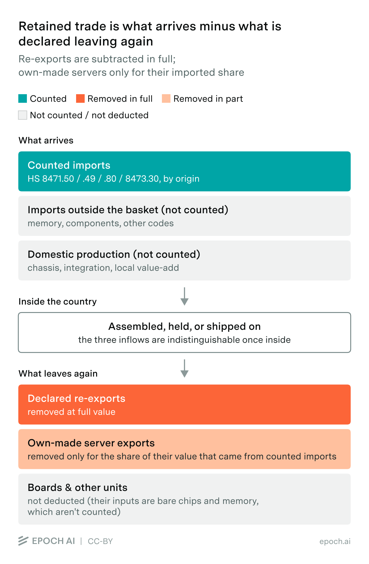
The principle is that each accelerator should be counted once, at the market where it is finally deployed. Gross customs imports break that rule in four ways. The same correction applies to every country’s records:
| What goes wrong | The correction | Affected countries |
|---|---|---|
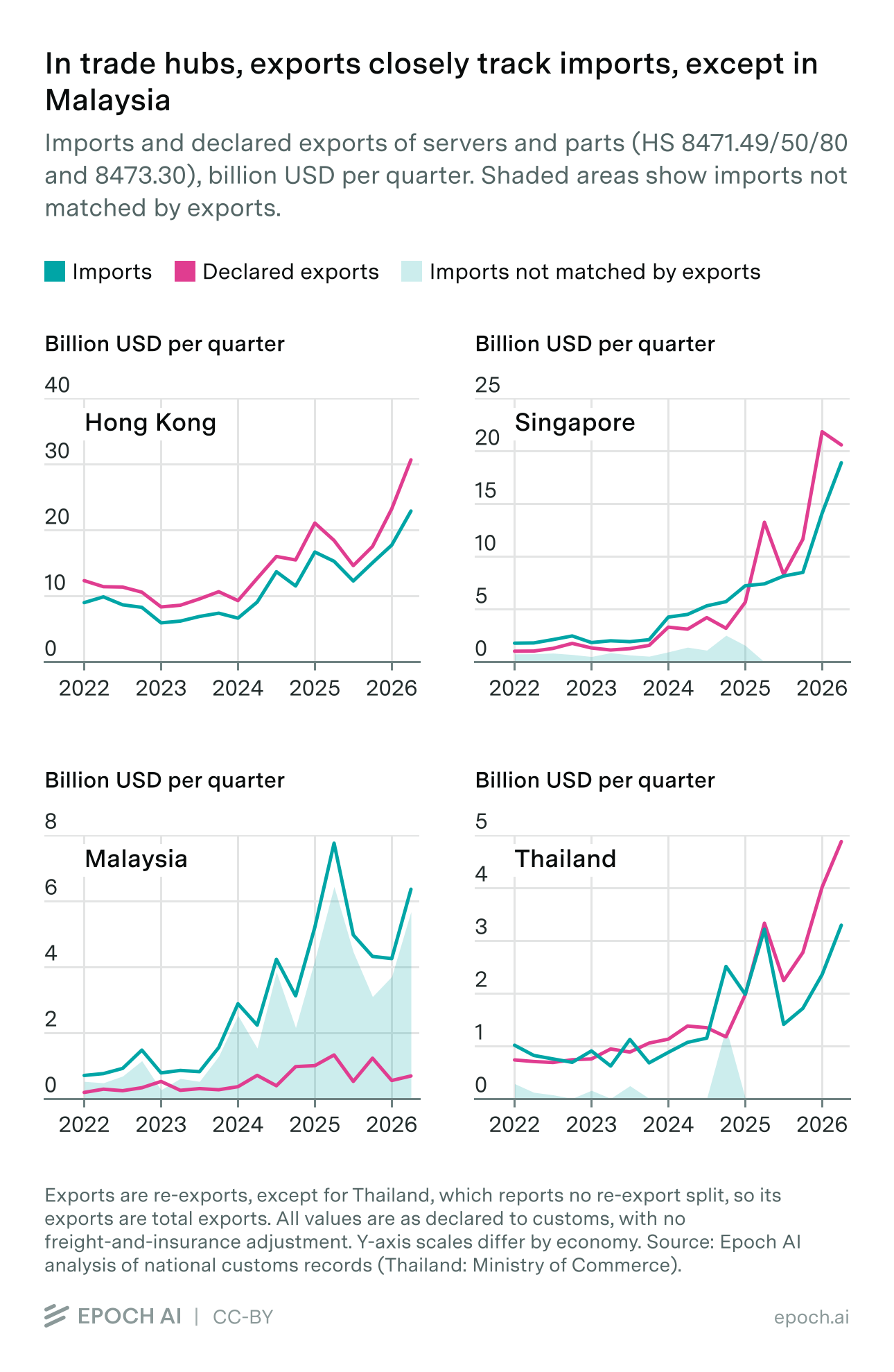
| Pass-through. Entrepôts import and re-export the same goods, so counting hub imports as consumption double-counts everything that moves on. | Subtract the goods the country itself declares as re-exports, at full value. | US, Hong Kong, Singapore, Malaysia, Canada; the EU and the UK through production statistics (below) |
| Assembly round-trips. Parts flow into an assembly economy and return as finished hardware, so the same silicon is counted twice, once as boards into the assembler, again as servers into the final market. | Subtract the imported content of the servers a country builds and exports (below). | All; it matters for the US, Mexico, Malaysia, Thailand and China |
| Own goods coming back. A country’s own exports that return to it, through bonded logistics zones for example, never left economically. | Exclude arrivals whose declared origin is the importer itself. | All; in practice China |
| Mid-chain component crossings. Bare chips cross borders en route to packaging and assembly, not to be deployed. Korea imports $135B of bare logic (8542.31) against $46B of finished hardware; counting chip-form crossings would make it a top-three compute holder because of its HBM business. | Exclude 8542.31 (bare chips) from every country: deployed compute makes its last crossing as a board or a system. | All |
Removing freight and insurance costs
Import values include the cost of getting the goods to the border; export values, and Epoch’s sell-in dollars, do not. We therefore adjust import values to exclude freight and insurance before comparing them with exports or chip sales, using the same method across countries. The US is the one country that publishes both values for every import line, together with the shipping weight, so we measure the freight-and-insurance margin there and apply it everywhere else.
The US data show that the margin depends mainly on how valuable the goods are per kilogram. Cheap, heavy goods pay a lot relative to their value and dense goods very little: shipments worth under $100 per kilogram pay 2.3% of their value, shipments at $1,500–3,000 per kilogram pay 0.45%, and above $12,000 per kilogram under 0.1%. Distance adds nothing once density is accounted for: at the same density, servers from Taiwan, Vietnam and the Czech Republic pay much the same per kilogram. The margin does move with the freight cycle, from 1.5% of value in 2022 at the post-COVID air-cargo peak to 0.8% in 2024 and back to 1.2% in early 2026.
We fit that as a curve, where \(v\) is the value density in dollars per kilogram and \(a_q\) is a level for quarter \(q\):
\[\text{margin}_q(v) = a_q \, v^{-0.39}\]The exponent is measured once, on the whole 2022–2026 sample of about 26,000 code × origin × month cells; the level is refitted each quarter from that quarter’s cells alone, so it follows the freight cycle without any quarter borrowing from another. Every import row of every country that reports landed values (all but the US, Mexico and Canada) is then divided by one plus the margin. Australia’s Comtrade imports are reported CIF and receive this adjustment. A row’s own value per kilogram sets its margin where the country reports weight (China, the EU, Korea, the UK, Indonesia, Thailand and part of Japan); otherwise the row takes the value per kilogram of the same code and quarter across the countries that do report weight (Malaysia, Singapore, Hong Kong, India and the rest of Japan). For a GPU server at $400 per kilogram the margin runs 0.9–1.6% of value depending on the quarter; for dense boards at $2,000 per kilogram, 0.5–0.9%. Over the AI window this removes about $30 billion from the import records, most of it in the EU, Hong Kong and China, and moves the headline ratio by about 0.3 points.
Netting mechanics
Three mechanics then apply throughout, per code and month:
- Carry. An export deduction that exceeds current imports is carried forward rather than discarded. Netting starts in January 2021, so the published 2022 estimates inherit the preceding year’s balances. A separate quarterly rule can revise previously counted excess when a later shortfall occurs; Section 3.3 explains that charge-back.
- Imported content of exported servers. A country that builds servers from imported boards and ships them out has sent the boards on in a different form. We subtract those exports at the share of their value that was imported, and we read that share from how heavy the exported machines are per dollar. Light, expensive machines are mostly imported accelerators; heavy, cheap ones are mostly locally assembled metal and CPUs. A server exported at $250 per kilogram nets 10% of its value, at $600 per kilogram 40%, at $2,000 per kilogram 90%. If the weight of the exported machines is not available we take the same share from their value per unit, and if neither is available we use the accelerator share found in the country’s own imports of that code. The deduction is taken first from that month’s imports of the same code, and any remainder from the country’s other counted import lines in proportion to their size. Exported boards and other units are never deducted: their inputs are bare chips and memory, which the basket does not count.
- Destinations without import records. We use selected exporters’ shipments to estimate arrivals in destinations whose own records are unavailable. These include hub re-exports, US domestic exports and selected finished-hardware exports from the EU, Malaysia, Singapore, Hong Kong, the UK, Indonesia and India, together with Taiwan’s residual destination coverage. These are gross trade values entering the baseline and content calculations, not amounts treated wholly as accelerator value.
Put together. For each country, code and month:
\[\text{retained} = \text{imports} - \text{own goods returning} - \text{declared re-exports} - k \times \text{own-made server exports}\]where \(k\) is the estimated imported share. Malaysia also receives the server mirror-gap deduction described below. A negative month carries into the next.
The table shows the netting calculation for each reporting country or bloc for the finished-hardware basket (847149/50/80 and 847330), in billions of dollars. Totals start in 2023Q3 and end at the last available month for each reporting country or bloc, so the endpoints vary across rows:
| Gross $B | Re-exports and own goods returning $B | Own-made server deduction $B (k) | Retained $B | Removed | |
|---|---|---|---|---|---|
| United States | 668.7 | 134.3 | 20.5 (45%) | 514.0 | 23% |
| China | 211.2 | 47.7 (own goods returning) | 9.6 (14%) | 153.9 | 27% |
| European Union | 157.6 | 59.7 | 7.6 (33%) | 90.2 | 43% |
| Hong Kong | 153.7 | 199.4 | 0.0 (28%) | 0.0 | 100% |
| Mexico | 138.4 | 0.0 | 149.1 (77%) | 0.0 | 100% |
| Singapore | 87.1 | 98.0 | 8.8 (68%) | 6.4 | 93% |
| Malaysia | 47.0 | 8.2 | 7.3 (38%) | 29.3 | 38% |
| South Korea | 35.6 | 0.0 | 0.3 (35%) | 35.3 | 1% |
| Japan | 30.2 | 0.0 | 0.2 (30%) | 30.0 | 1% |
| United Kingdom | 28.7 | 9.5 | 0.9 (48%) | 18.2 | 36% |
| India | 25.3 | 0.0 | 0.5 (54%) | 24.8 | 2% |
| Thailand | 19.9 | 0.0 | 6.4 (70%) | 13.5 | 32% |
| Canada | 18.5 | 1.3 | 0.4 (25%) | 16.8 | 9% |
| Australia | 16.1 | 0.0 | 0.1 (33%) | 15.9 | 1% |
| Indonesia | 9.7 | 0.0 | 0.1 (59%) | 9.7 | 1% |
| Saudi Arabia | 4.1 | 0.0 | 0.0 (59%) | 4.1 | 1% |
Across the reporting windows in this table, netting removes 42% of gross finished-hardware trade ($690 billion of $1,652 billion). Malaysia’s retained total includes the additional $2.04 billion server mirror-gap deduction, shown separately in the discussion below rather than in the own-made-server column. Mexico’s retained trade rounds to zero at this precision. Vietnam’s output is observed through its partners’ imports because the estimator has no Vietnamese destination customs dataset. Destinations without their own datasets are estimated from selected dispatch corridors.
Six cases are worth discussing in more detail:
- European Union. Netted as one bloc, because members are not self-contained: Hungary exports $12 billion of servers against $0.7 billion of extra-EU imports, since its inputs arrive from stock cleared in the Netherlands. The re-export share of each member’s exports comes from its own statistics. What it reports producing itself, in Eurostat’s PRODCOM survey, sets the floor of own-made goods, and its imports cap what it can have re-exported. The Netherlands and Ireland re-export essentially everything they ship out and Germany 95%; Hungary, Czechia and Poland assemble rather than trade, at 4%, 20% and 10%. Weighted together, 58% of the EU’s server exports are re-exports.
- South Korea. Korea follows the same netting rule as other destinations. Its exports under these codes are dominated by memory modules on the parts line, whose own-made exports are not deducted. Explicitly labelled imported DRAM modules receive zero accelerator content in the classification step; other products retain their classifications from national tariff categories or physical measurements (Section 3.4).
- Malaysia. An assembler and a hub at once. Its $8.2 billion of declared re-exports are deducted at full value, and its own-made server exports are deducted at their estimated imported-content share of 38%, or $7.3 billion. We additionally deduct 50% of the positive China–Malaysia server mirror gap, by code and calendar quarter on the FOB basis. This adds a $2.04 billion deduction over the table’s reporting window and leaves $29.3 billion of retained trade. The quarterly gap is distributed over China’s recorded monthly arrivals in proportion to their value, then passes through the existing negative-carry rule. The same rule applies in 2021; no gap is deducted for boards or other units, and China receives no additional credit. Zero and full deductions are structural alternatives without assigned probabilities.
- Mexico. Export k uses the chip-content estimate for imports as a fallback. A supplementary INEGI dataset provides monthly quantities and weights for January 2023–June 2026 across nine corridors plus a World total, and annual observations for 2022–23. Its 5,218 overlapping trade values match the estimator’s input data exactly. Sensitivity tests use these physical fields, but they do not reliably distinguish ordinary-computer assembly from accelerator assembly, so the baseline estimate uses the import-content fallback.
- Thailand. Thailand does not separate re-exports from its own exports, so every export counts as own-made. Exported servers are deducted at the imported-content share implied by their physical evidence, rather than at full value.
- The other final markets. Japan, India, Indonesia, Australia and Saudi Arabia export little on these codes, and the deduction removes 1–3% of their gross imports. Canada declares its re-exports, which are deducted at full value, 9% of its gross imports in all. The UK is a distributor: its production statistics (the ONS ProdCom survey) say it makes little of what it ships, so 76% of its exports are deducted as re-exports, 36% of its gross imports in all; they go to the Netherlands, Germany, the US, Iceland and Ireland.
Known weaknesses
- China, Korea, Japan, India, Indonesia, Thailand, Mexico, Saudi Arabia and Australia do not separate re-exports from their own exports, so every export from them counts as own-made. A server that passed straight through one of these countries is deducted at its imported-content share rather than in full, and a board that passed through is not deducted at all.
- Undeclared outward shipments may remain counted in the country they leave. The Malaysia server-gap adjustment addresses one observed discrepancy, but the 50% deduction is a modelling judgement and does not identify every onward shipment.
- The imported-content share k depends on assumed relationships between export value density, unit value and imported components. Those measurements can imply different shares: US export weights suggest about 45% imported content, compared with about 79% from unit values. The probability model varies export-evidence k by up to ±10 percentage points through shared and country-specific shocks. Where k is derived from import content, it moves with that content estimate (Section 4.5).
- For Mexico and Canada, the baseline export deduction uses import-content estimates where usable export physical evidence is absent. The Mexican sensitivity analysis illustrates the uncertainty in this fallback: more detailed physical fields can change the deduction without resolving the underlying product mix.
- Exporter coverage is incomplete. China, Korea, Japan, Thailand, Mexico, Saudi Arabia, Australia and Canada do not contribute additional export corridors to inferred destinations. Included shipments undergo baseline subtraction and accelerator-content classification, but neither step establishes that the hardware remains locally. Export declarations from different stages of a supply chain may also overlap.
- The EU members’ and the UK’s re-export shares assume their export mix to the rest of the world matches their total mix, and for Hungary, Czechia and Poland the share is an estimate from the import cap.
- The freight margin is measured on US shipping weights, which include packaging, while the other countries report net weight. Their goods therefore look denser than they are and the margin taken off them is slightly too small, by under a tenth of a percent of value. Goods that arrive by truck from a neighbour, the UK’s imports from the EU or Singapore’s from Malaysia for example, are charged a margin they did not pay, about 1% of those flows.
3.3 Step 2: separate AI trade from ordinary trade
There is no product code for AI hardware. The codes we use carry plenty of goods that have nothing to do with AI (racks of ordinary web servers, standard logic and memory modules), and netting in step 1 does nothing about that, because those goods really did arrive and really did stay. So we cannot treat every netted dollar as AI. We have to model the part that isn’t.
How the baseline works
For each destination and code, the reference starts with total retained trade in 2021 divided by twelve. We scale that monthly amount using the relevant index, normalized to its mean in 2021. Systems follow a client-IT index; boards and parts follow a selected-origin component index. Excess above the reference is candidate accelerator-related trade, whose content is assessed in step 3. The component reference is not an independently identified measure of non-AI trade.
In formula terms, for each destination–code series and month \(t\):
\[\text{baseline}(t) = \frac{R_{2021}}{12} \times \frac{I(t)}{\bar{I}_{2021}}\]\[\text{excess}(t) = \text{retained}(t) - \text{baseline}(t), \quad \text{netted over quarters}\]- \(R_{2021}\) (anchor): total retained trade for the destination–code series in 2021. It is computed after the trade deductions in step 1, and divided by twelve to give a monthly amount.
- Reference-year AI: we assume AI trade in 2021 was negligible for this calculation and apply no separate accelerator-sales carve.
- \(I(t)\): the destination–code reference index, normalized by its 2021 mean \(\bar{I}_{2021}\). Systems use the client-IT proxy; boards and parts use the selected-origin component reference.
- \(\text{excess}(t)\): retained imports above the reference, before chip-content classification. A month below its reference counts as negative; the quarterly ledger determines whether nearby surpluses offset it.
How quarterly offsets work
Monthly trade fluctuates around the baseline, so counting only the months above it would overstate AI trade. We keep a quarterly ledger for each destination and code instead. A quarter below its baseline can be offset by surpluses in the next two quarters, and can reduce surpluses counted in the previous two. A shortfall that isn’t offset within two quarters expires. As a result, the latest two quarters can still change as new data arrive.
Why we use 2021
We assume accelerator trade in 2021 was small enough to treat as negligible relative to ordinary trade in the counted codes. We therefore make no separate deduction for AI hardware in the baseline year. This avoids calibrating the reference using an estimate of 2022 accelerator sales, but it remains an assumption rather than a claim that no accelerators traded in 2021.
Both trade netting and the excess ledger begin in January 2021. That year supplies the baseline and warm-up history; it is excluded from published AI arrivals. Destinations estimated from exports use the same 2021 reference across all contributing sources, including Taiwan. Each annual reference is divided by twelve, with unrecorded corridor months entered as zero.
The UK’s historical reference. Changes in UK–EU reporting around 2021 make the raw series unsuitable for a consistent baseline. We reconstruct UK imports from the EU using EU exports to the UK, calibrated against July 2022–June 2023. The machine codes 847149 and 847150 are pooled for this reconstruction.
The UK client-IT index uses a consistent dispatch basis. For the parts index, we estimate the eligible-origin share of EU dispatches from the reconciled origin-by-dispatch data for the second half of 2022 and apply that share to 2021. This assumes the origin mix was stable enough for the backcast. Current UK trade observations continue to use UK records.
How the index is built
The reference differs by code because finished systems and components have different demand and pricing cycles.
-
For the systems codes (8471.49/50/80), we use the reporter’s own imports of laptops and desktops (8471.30 and 8471.41), computer monitors (8528.51/52), printers (8443.31 and 8443.32) and input/output units (8471.60), using the codes available from each source. The assumption is that these track the ordinary-computing cycle without directly counting accelerators. The indices capture the post-COVID client-IT downturn and subsequent recovery; their levels are normalized to 2021.
-
For boards and parts (8473.30), we use the reporter’s imports of the same code from selected origins as a component reference. This avoids imposing the client-IT cycle on components. Origin selection does not identify products: the reference can include ordinary computing, standalone memory, AI-related component demand and accelerator hardware.
Finished memory modules share 8473.30 with other computer parts, including accelerator boards. The component index can therefore respond to memory prices and product composition as well as volumes. Rising reference values are observed movements in this selected-origin trade, not a separately measured correction for memory inflation.
Destinations whose customs records we do not hold follow their own Comtrade version of the same index where we have pulled one (12 destinations), and the world average of the measured indices otherwise.
How much retained trade counts as AI-related
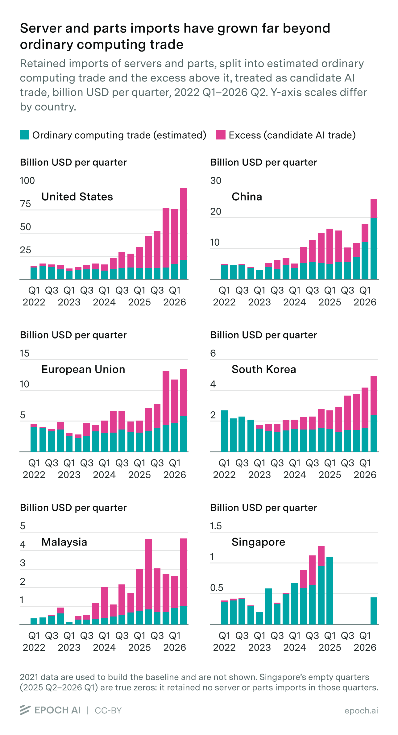
The table decomposes the reference adjustment over calendar arrival quarters 2023Q3–2026Q2. “Full window” covers 2022Q1–2026Q2; 2021 is used only for the reference and warm-up. Values are billions of dollars.
| Destination | Retained trade, full window ($B) | Excess, full window ($B) | Retained trade, 2023Q3–2026Q2 ($B) | Excess, 2023Q3–2026Q2 ($B) | Share removed by baseline |
|---|---|---|---|---|---|
| United States | 600.8 | 380.1 | 514.0 | 362.2 | 30% |
| China | 180.6 | 74.2 | 153.9 | 71.3 | 54% |
| EU | 113.2 | 49.4 | 90.2 | 46.1 | 49% |
| Malaysia | 32.0 | 22.6 | 29.3 | 22.0 | 25% |
| South Korea | 48.1 | 17.9 | 35.3 | 17.2 | 51% |
| United Kingdom | 23.9 | 10.6 | 18.2 | 9.5 | 48% |
| Japan | 41.0 | 9.9 | 30.0 | 9.0 | 70% |
| Australia | 20.3 | 8.6 | 15.9 | 8.2 | 49% |
| Canada | 23.0 | 7.4 | 16.8 | 6.8 | 60% |
| India | 32.2 | 9.8 | 24.8 | 9.1 | 63% |
| Indonesia | 12.2 | 7.5 | 9.7 | 6.6 | 31% |
| Singapore | 8.7 | 1.2 | 6.4 | 1.1 | 82% |
The reference and quarterly offsets remove different shares of retained trade across destinations. Over 2023Q3–2026Q2, the reduction is 30% for the US, 54% for China, 49% for the EU and 51% for Korea. It is 70% for Japan, 63% for India and 60% for Canada. Malaysia’s reduction is 25%, while Singapore’s is 82%. These differences depend on the 2021 reference, subsequent index movements and the quarterly offsets; they do not directly identify the products in the remaining excess.
Alternative baselines we tested
- Historical fixed-growth test. The following reference alternatives were evaluated under the earlier 2022-reference specification. Growing that reference at 0%, 5% or 10% a year failed to capture the post-COVID fall in ordinary IT trade. These tests motivate a changing reference, but their numerical results are not comparisons of the current 2021 estimator.
- Changing the placebo basket. Three variants were computed, each leaving the boards placebo and everything downstream unchanged:
- Systems from non-AI origins. Imports of the same systems codes, restricted to origins outside the AI assembly geography. This is the closest the data comes to measuring non-AI servers directly, but the exclusion list cannot keep up with where AI servers are actually assembled. By 2025–26 the US version of this placebo is dominated by Hungary, Ireland and Czechia, all of which ship AI servers, so this reference includes some of the AI trade we are trying to estimate.
- Laptops and desktops only. This narrower basket excludes monitors, printers and input/output units. Laptops account for about 70% of the composite basket’s value, so the two indices track each other closely.
- Client-IT peripherals only. Monitors and printers alone (8528.51/52 and 8443.31/32). These share the demand cycle and logistics of client IT but contain no compute and almost no memory, so they cannot inherit the 2025–26 memory repricing. Their 2023 dip (annual means of 0.78 for the US, 0.82 for the EU, 0.82 for Korea) confirms the downturn was broad client IT rather than something specific to laptops and desktops.
How the choice of baseline changes the estimate
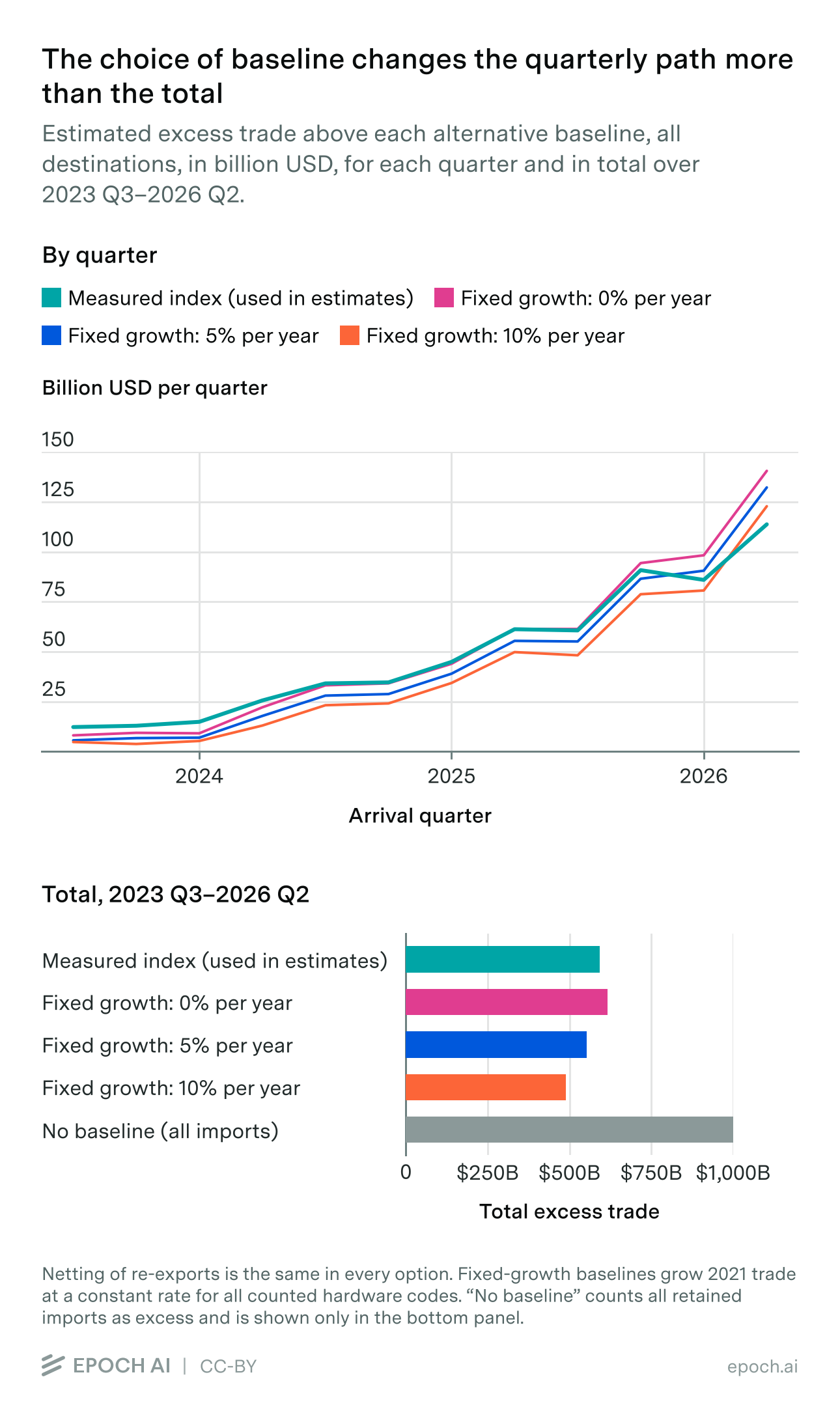
Over calendar arrival quarters 2023Q3–2026Q2, the indexed 2021 reference leaves $592 billion of excess trade. Fixed annual growth of 0%, 5% and 10% leaves $616 billion, $553 billion and $489 billion, respectively. With no reference subtraction, retained trade totals $1,003 billion. These are trade dollars before the accelerator-content adjustment, not chip-dollar estimates.
In the 2023Q3–2024Q1 trough, the indexed reference leaves $12–15 billion a quarter above the baseline, compared with $6–7 billion under 5% fixed growth. The measured index lowers the baseline during the ordinary-IT downturn, leaving more of the observed imports above it.
In recent quarters, rising component values increase the boards reference faster than the fixed-growth alternatives. The data do not separately identify how much of this movement reflects memory repricing, other component demand or accelerator trade.
The alternative-basket tests described above are not included in this chart, because they do not yet have consistent 2021 histories. This comparison uses current netting and changes only the reference used to calculate excess trade.
Baseline specification
The baseline estimate uses the measured index of gross placebo imports. A historical re-export-netting test for the US, Hong Kong and Malaysia increased chip dollars by 0.215% against matched gross controls and moved no country share by more than 0.079 percentage points. Hong Kong’s small net residual was unstable and reached the index floor in nine smoothed months. These results support using gross imports for the placebo basket; the test covers neither every country nor the boards’ origin-based index. The uncertainty model perturbs the measured baseline around its reference path (Section 4.5). The structural envelope also tests a flat systems reference and a client-IT reference for boards, crossed with alternative content assumptions. Other fixed-growth and basket comparisons remain separate sensitivity tests.
The chart above stops at excess trade dollars. Section 3.5 compares the same current-reference alternatives with chip sales after accelerator-content conversion. The earlier alternative-basket tests remain historical.
Known weaknesses
- The systems placebo assumes ordinary servers move with the client-IT cycle. While this seems to match our expectations (the 2023 downturn), it is still an assumption, as we can’t rely on any “non-AI server” product code directly.
- The US 2025 index partly measures tariff effects: if tariffs suppress non-AI imports the baseline correctly falls, but the index is then entangled with trade policy, not just the IT cycle.
- The two-quarter offset window is a judgement call. A shorter window leaves more temporary fluctuations counted as retained excess; a longer one allows later weak trade to erase earlier arrivals. Recent quarters can consequently be revised when new observations arrive. Starting the ledger in 2021 reduces the artificial boundary at the start of the published 2022 series, but does not recover balances from before the available history. Charges reduce the original surplus quarter, so the comparison and allocator do not differ because a later negative contribution is discarded.
3.4 Step 3: estimate the AI chip share of trade value
The excess from step 2 is trade value attributed to AI hardware, not necessarily accelerator value alone. An HGX server reference configuration priced at $285k contains about $208k of accelerator modules; other value belongs to CPUs, host memory, storage, networking, chassis and integration. The accelerator basis includes the module’s HBM and packaging. We multiply excess dollars by an estimated accelerator-content share to make the comparison with the narrower chip sales basis.
We estimate chip content separately for each combination of importer, origin and month, then apply the resulting monthly share to the destination’s excess from step 2. Where a country’s tariff codes identify the product, we use them; for example, memory modules in Japan, South Korea and the US get no chip value. Otherwise, we compare the declared value per unit, or per kilogram where unit counts have insufficient coverage, with reference prices for accelerator boards and servers. Those reference prices come from our chip prices and product mix, which makes this the step where the customs estimates depend most on our sales data.
-
Family constants and the product mix: each accelerator family gets its own content constant, and the constants are weighted by the quarterly product mix in chip sales to give the share for hardware that arrives as complete systems.
System type Chip content Basis HGX servers 0.73 $208k of accelerator in a $285k server GB200 / GB300 racks 0.79 Built up per generation, below TPU and Trainium systems 0.70 In-house chips (TPU, Trainium) are valued near production cost, so no margin uplift -
Rack configurations: chip content depends on the system configuration and its valuation. A GB200 NVL72 reference has 72 GPUs at about $37k each: $2.66 million of modules in a $3.1 million rack, or 0.86. A GB300 reference has 72 at about $43k: $3.10 million in a rack just under $4 million, or about 0.79. The estimator uses 0.79 for the rack benchmark. Appendix A specifies the content perturbations used in the uncertainty model.
-
Reading each cell: every combination of importer, origin and month is a cell (importing member, origin and month for the EU), and each is read from its own records. Where the number of units is available for at least 90% of the cell’s value, we divide dollars by pieces and compare the result with the accelerator price available in that market: roughly $12k for an H20 and $30k for an H800 on the China side, around $33k elsewhere. That price is the average across the models on sale, so a board carrying one of the cheaper models, or one declared at cost between related companies, can arrive at a third of it and still be one accelerator. The boards band therefore starts at 0.35 times the reference. The table gives the reference points used to assign accelerator-content shares; intermediate values are interpolated.
Dollars per unit What is crossing Content share Under 15% of the accelerator price Ordinary electronics 0.05 A third to 2.5 times it Accelerator boards 0.93 More than five times it Complete servers The product-mix share above When piece counts do not meet the coverage rule, the classifier uses dollars per kilogram where available. The assumed boards ramp rises from 0.05 at $1,000/kg to 0.93 at $3,000/kg; the machines ramp rises from 0.05 at $600/kg to the eligible system-mix share at $2,000/kg, with log-linear interpolation. These are classification assumptions, not product-identification tests: valuable memory can have densities similar to accelerator boards. Each monthly cell is weighted by its positive excess above its own 2022 pace. We use unsmoothed monthly content when classified excess reaches $50 million/3 (about $16.7 million) and the selected physical field covers at least 90% of that month’s value. With insufficient monthly evidence, we retain the existing quarterly reading (a three-quarter median), then the pooled prior for that destination and code. Where physical data provide no content estimate, machines use the eligible product mix and boards receive the default share of 0.93. Native tariff-code content weights are also monthly; explicitly identified memory stays at zero.
Historical quarterly diagnostics illustrate the scoring rule. Boards arriving in China from Vietnam in 2024Q3 were declared at about $2,100 per kilogram, between the two density anchors, implying a score of 0.66. Boards arriving in Malaysia from Taiwan through 2025 were declared at $460–740 per kilogram, below the lower anchor, implying 0.05. These pooled examples explain the classifier; the baseline estimate applies it to each month’s evidence without smoothing where the monthly gates are met.
The classifier assigns different effective content scores to different observed mixes. Low-value server cells receive low scores, while ambiguous parts can fall well below the 0.93 accelerator-board benchmark.
-
National tariff lines take precedence where their definitions identify product scope. We assign no accelerator value to separately identified standalone memory modules in Japan, the US and South Korea. HBM and packaging already included in an accelerator’s selling price remain in scope. The three memory-module codes are listed below.
| Reporter / flow | National code | Definition |
|---|---|---|
| Japan imports | 847330011 | DRAM chips mounted on a circuit board with terminals for connection to computers or their units; supporting components may be present. Japan’s export code is undivided. |
| South Korea | 8473304060 | DRAM modules, classified as computer parts and accessories. |
| US imports | 8473301140 | Memory-module printed-circuit assemblies for use principally or exclusively with computers; not limited to DRAM. |
Japan’s module and remainder cells preserve each origin-month’s total FOB value, allocated using the national tariff lines’ declared-value shares, with quantities and weights kept in their own groups. This separates identifiable memory before estimating content in the remainder. Identified memory modules remain in the trade totals used for netting but contribute no accelerator dollars. Broad non-memory categories can still contain heterogeneous products.
How much of the excess is accelerator value
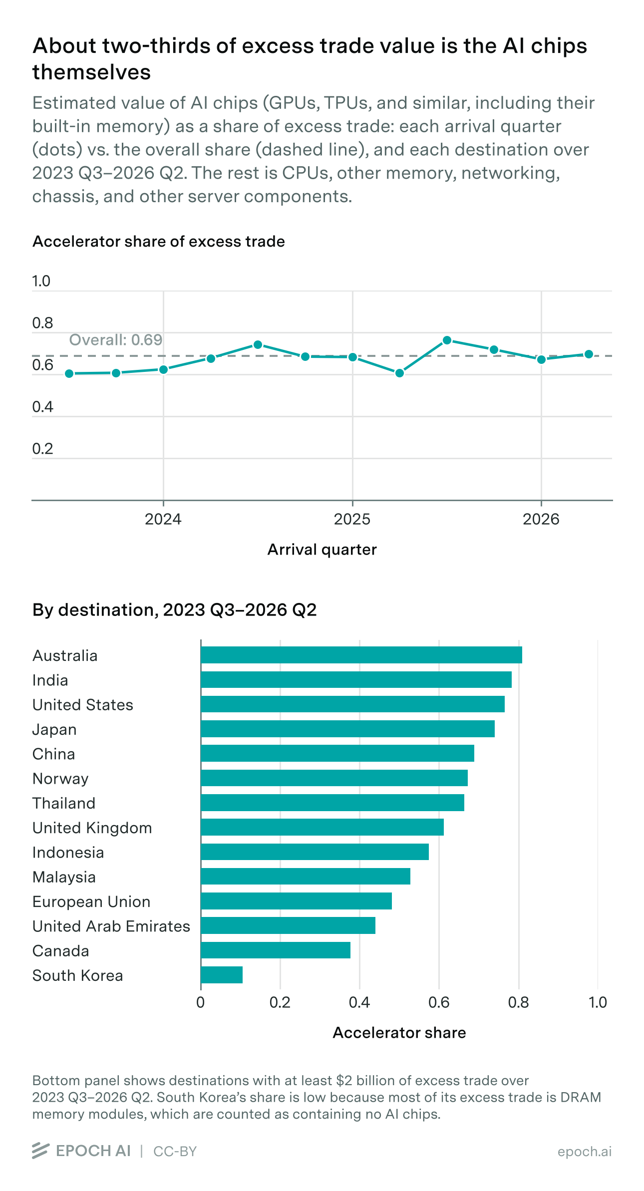
Over calendar arrival quarters 2023Q3–2026Q2, $592.0 billion of excess trade becomes $408.2 billion of accelerator dollars, an effective content share of 0.69. The table covers destinations with at least $2 billion of excess trade over that window.
| Excess, AI window $B | Chip, AI window $B | Chip share | |
|---|---|---|---|
| United States | 362.2 | 277.3 | 0.77 |
| China | 71.3 | 49.1 | 0.69 |
| European Union | 46.1 | 22.2 | 0.48 |
| Malaysia | 22.0 | 11.6 | 0.53 |
| South Korea | 17.2 | 1.8 | 0.11 |
| United Kingdom | 9.5 | 5.8 | 0.61 |
| India | 9.1 | 7.1 | 0.78 |
| Japan | 9.0 | 6.7 | 0.74 |
| Australia | 8.2 | 6.6 | 0.81 |
| Canada | 6.8 | 2.6 | 0.38 |
| Indonesia | 6.6 | 3.8 | 0.57 |
| Norway | 3.3 | 2.2 | 0.67 |
| Thailand | 2.8 | 1.9 | 0.66 |
| United Arab Emirates | 2.7 | 1.2 | 0.44 |
Effective shares range from 0.11 for Korea, after explicit DRAM-module exclusion, to 0.81 for Australia. The US is 0.77, Japan 0.74, the EU 0.48, Canada 0.38 and Malaysia 0.53. These averages pool monthly readings over 2023Q3–2026Q2 and remain estimates of product composition.
Countries without import records
For destinations without usable import records, we classify exporter–destination–code–month observations. Machine codes use value per piece where pieces cover at least 90% of the cell’s value; otherwise they use value per kilogram where weight meets the same coverage rule. Boards use weight. The existing price and density rules apply without smoothing.
We distribute the destination’s monthly net excess across exporters in proportion to their gross shipment values, then apply the content estimates. We do not add together separately clipped positive excesses from each exporter.
Where physical fields are missing, uncovered value receives the value-weighted mean content of observed shipments from the same exporter, code and quarter, using a donor pool with at least three destinations. If that pool is unavailable, we broaden it to the same code and quarter, then the same code and year. The pools include ordinary low-content goods. China and Hong Kong are excluded as donors because their classifications use a different price reference. If no suitable pool exists, the run stops rather than substituting an accelerator-system share.
Covered value retains its own physical classification. We report how much of each destination’s estimate depends on imputed content; that dependency is not a probability that the estimate is wrong.
Matching arrival dates to sales dates
Customs records show when chips arrive, and our sales data show when they’re sold. We spread each quarter’s sales evenly across its three months and shift them two months later. April–June arrivals are therefore matched to February–April sales: two-thirds of Q1 sales and one-third of Q2 sales. Because our sales data start in January 2022, the first arrival quarter includes only March arrivals. The two-month delay is an assumption rather than a measured shipping time, and actual delays likely vary by country and over time.
The allocator uses the same calendar arrival quarters as the dollar comparison. Incomplete customs quarters are excluded. Missing or incomplete source-sales windows are flagged. Timing can still differ by country and period.
Known weaknesses
- The price thresholds, density ramps and coverage rules are judgement calls. The probability model varies the unit-price and density thresholds and selected server/board content readings; the 90% coverage rule is fixed. Prior widths express modelling judgement rather than empirically estimated classification error (Section 4.5 and Appendix A).
- The pieces and weights describe a cell’s whole flow, but the share they produce is applied only to the excess above the baseline. A cell that mixes AI servers with ordinary servers from the same origin shows a unit value between the two, and its share is wrong in proportion to the mix. Cutting the data by origin and month, and giving each cell weight only for its excess, limits this but cannot separate the two kinds of hardware when they travel together. The physical composition of the netted residual is not separately reconstructed.
- The negative-control test using national tariff labels demonstrates the identification problem: hiding the labels on explicitly identified Korean memory lines makes the density ramp assign about 91% accelerator content on average. Classifications based on national tariff labels exclude those known memory lines; broad codes without equivalent labels remain ambiguous. China’s collected 847330 data do not provide an equivalent memory-module split. The structural envelope tests alternative readings of ambiguous 847330 parts and 847180 units, alongside alternative baseline constructions, server-mixture and selection assumptions, and Malaysia mirror-gap deductions (Section 4.5).
- Within measured importer datasets, boards without usable physical or national-code evidence can still receive the 0.93 fallback. Destinations inferred from exports instead use observed-shipment imputation. Neither approach resolves product mixtures hidden within an average unit value or density.
- The piece counts and weights are taken as declared. They are filled in by the filer, are not checked by customs the way values are, and the two sides of a border do not always agree on them. Where we have doubts about a declared count or weight we do not correct it; we can only choose which of the two to use.
3.5 How the estimates compare with chip sales
We compare calendar-quarter customs chip dollars with chip sales interpolated into the same arrival quarters under the two-month lag. The full AI comparison covers 2023Q3–2026Q2 arrivals; the recent comparison covers 2025Q1–2026Q2.
| Metric | Full AI period | Last 6 quarters |
|---|---|---|
| Cumulative match | 103.4% | 109.6% |
| Median quarterly match | 98.4% | 107.3% |
| Mean absolute percentage difference | 14.6% | 12.4% |
Cumulative match divides total customs chip dollars by total corresponding sales dollars. Median quarterly match is the median of the quarterly ratios. Mean absolute percentage difference averages the absolute quarterly gaps relative to sales. These measure discrepancies against chip sales, not errors against known truth.
Why the quarters diverge
Customs invoice values and the model prices in chip sales need not move together. Price changes can alter the dollar comparison even at unchanged physical quantities, while changes in product mix, assembly geography and shipment timing can also move it. HBM is part of the accelerator module itself; other memory sits outside it in the host system. The evidence does not identify a unique explanation for the quarterly discrepancies.
The historical early undershoot coincided with low unit values for boards crossing into the US, at 40–90% of the chip sales ASP before rising in later quarters. One possible explanation is that hardware entered at intercompany cost and was sold to final customers after the border, depressing customs dollars relative to sell-in prices. Product mix and classification error remain alternative explanations; this observation does not identify a correction.
We have not established what causes the later overshoot. A fixed per-model ASP can miss market-price changes within a model’s life, including changes in the value of integrated HBM. Assembly moving outside Taiwan may also change the lag between sell-in and the final observed crossing. The historical price observations and Taiwan-side comparison motivate these hypotheses, but neither establishes their size or rules out content-classification and product-mix errors.
How the baseline choice affects the match with chip sales
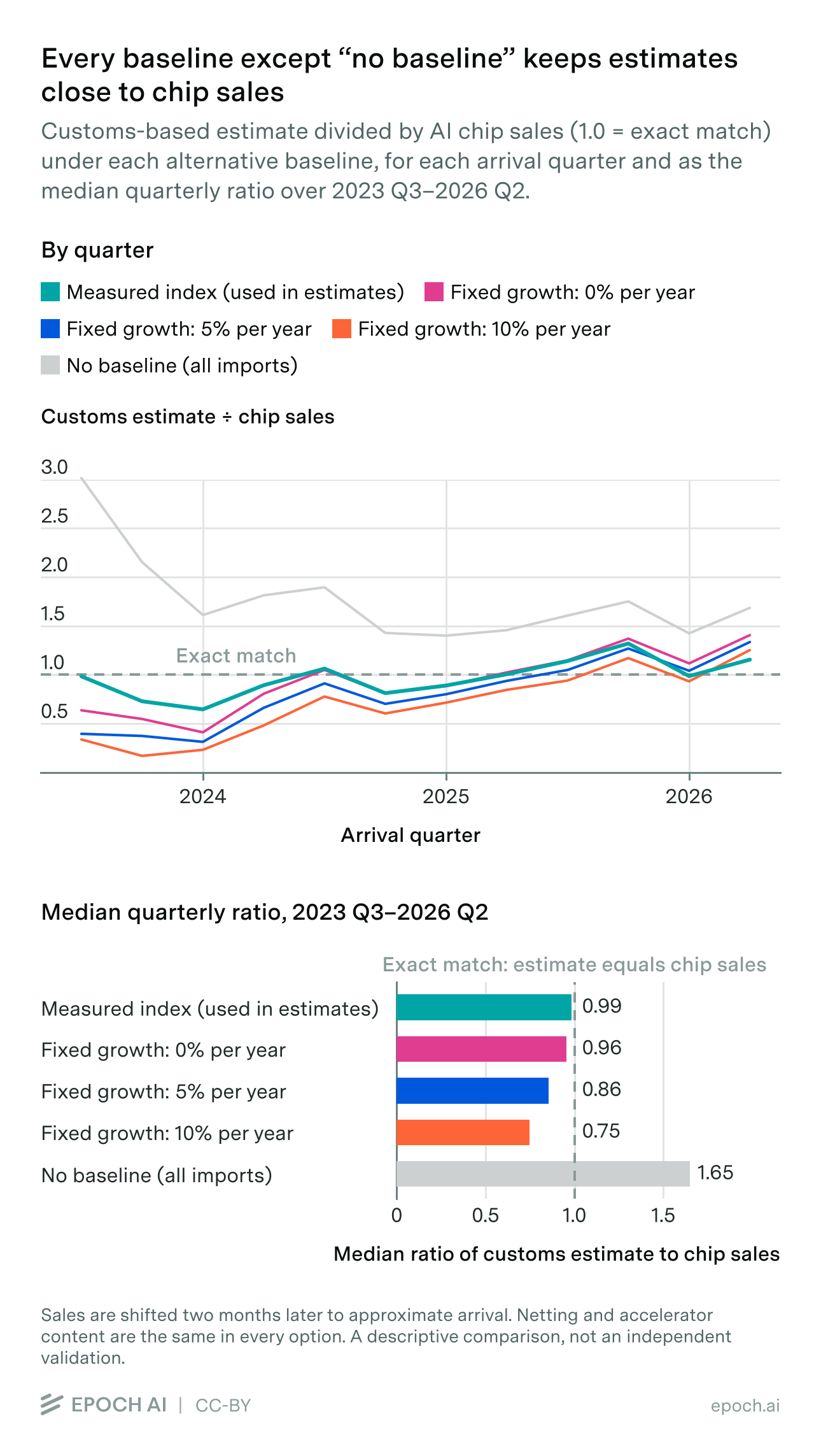
The October 19, 2026 rerun uses the 2021 reference and calendar arrivals with a two-month sales lag. Over 2023Q3–2026Q2, median quarterly customs-to-sales ratios are 0.99 for the indexed reference and 0.96, 0.86 and 0.75 for fixed annual growth of 0%, 5% and 10%. Without reference subtraction, the median is 1.65. Netting and physical content evidence are held fixed across these comparisons. The alternative-basket lines are omitted because they do not yet have consistent 2021 histories. This rerun includes the Australia historical-value and Singapore piece-coverage corrections; it is a descriptive sensitivity test, not independent validation or a rule for selecting the baseline.
Known weaknesses
- The early undershoot and late overshoot have plausible explanations, not a uniquely identified correction. The baseline method does not adjust them away or choose parameters to eliminate the discrepancy.
- The two-month lag is one global convention, not a measured timing rule for every shipment. Assembly, freight, customs recording and deployment delays can vary by destination and period. The improved fit does not establish that the same lag will remain appropriate out of sample.
4. Allocating chips to countries
Our chip sales data estimate how many chips of each model are sold each quarter, and the customs data estimate where AI chip spending goes. We combine the two to estimate how many chips of each model arrive in each country.
4.1 How chips are divided among countries
We first estimate how many chips of each model arrived worldwide in each quarter, using chip sales and the assumed two-month delay. We then divide those chips among countries according to their shares of customs-derived accelerator dollars, subject to the model eligibility rules below. The country estimates add up to the worldwide total for each model.
The latest complete customs quarter is April–June 2026. Under the two-month lag, its sales budget covers February–April. Cumulative arrivals through June therefore include all recorded sales from 2022Q1 through 2026Q1, plus one-third of 2026Q2 sales. Residual-country splits and EU member allocations use the same calendar customs quarters.
The series begins with sales recorded in 2022, so its first arrival quarter includes only the March arrivals attributed to January sales. Missing or incomplete source-sales windows are flagged, and incomplete customs quarters are excluded.
Not every model can go everywhere, so units are split into three pools before distribution:
- China-fabbed models (Huawei, Cambricon) never appear in Taiwan-supply-chain trade data, so they are allocated to China outright.
- China-market variants (A800, H800, H20, MI308X, i.e. the models designed for lawful sale to China) are split across China and Hong Kong by their corrected dollar shares, which in practice means China.
- Everything else, the global pool, is allocated across all destinations by their share of corrected chip dollars, after netting out of China’s dollars what the first two pools already absorbed. Within the pool every destination gets the same model mix, with some exceptions as described below.
We exclude allocations below one unit per destination-quarter and redistribute their dollars within the same pool. Each destination-quarter also carries an evidence score: its excess relative to the variability of its pre-window quarterly gaps between retained trade and the baseline, through 2023Q2. The noise scale has an absolute floor and a floor proportional to the mean baseline. Cumulative scores adjust for the number of quarters accumulated. The score is published alongside the estimate and is not used to remove allocations.
4.2 Which chips can go where
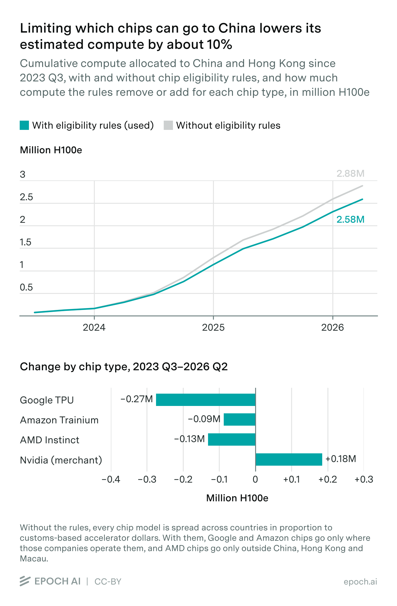
Without eligibility restrictions, proportional allocation assigns every global-pool model to every destination, including countries where we have no evidence that those models are deployed. Google’s TPUs and Amazon’s Trainium are not sold on the merchant market, so they can only sit where their designers operate them. AMD’s merchant volume is small and committed to Western hyperscalers. Over arrival quarters 2023Q3–2026Q2, an unrestricted rule would allocate China and Hong Kong 0.27 million H100e of Google TPUs, 0.09 million H100e of Amazon Trainium and 0.13 million H100e of AMD chips.
For these reasons, AMD’s models are allocated only across destinations outside China, Hong Kong and Macau, and Google’s and Amazon’s silicon to the eligible locations in our geography table: TPU v4, v4i, v7 and v8i and Trainium in the US alone; v5p in the US and the EU; v5e in the US, the EU, Japan, Chile, Singapore and Canada; v6e in the US, the EU, Japan, Chile, Singapore, India and Brazil. Within each model’s eligible set, shares are renormalized. China retains its dollar allocation, but within the global pool the model assigns those dollars to Nvidia GPUs assumed to reach China through diversion after export controls. The replacement is not one-for-one in units: captive silicon is priced near cost while merchant Nvidia carries the full margin, so the same dollars buy fewer chips. Over the same quarters, these eligibility constraints lower the cumulative China + Hong Kong allocation by about 10%: 2.58 million H100e against 2.88 million under the uniform mix. The withheld capacity is partly replaced by 0.18 million H100e of additional merchant Nvidia. These are allocation counterfactuals, not independently observed inventories.
TPU v8i is assigned to the US as a placeholder because the geography table has no public region evidence for it. This should not be read as a confirmed deployment location. About 31% of the US allocation in H100e comes from TPU and Trainium geography assumptions; about 39% of China’s comes from Huawei and Cambricon assigned to China. Customs shares determine the distribution of the remaining eligible supply.
4.3 The China price premium
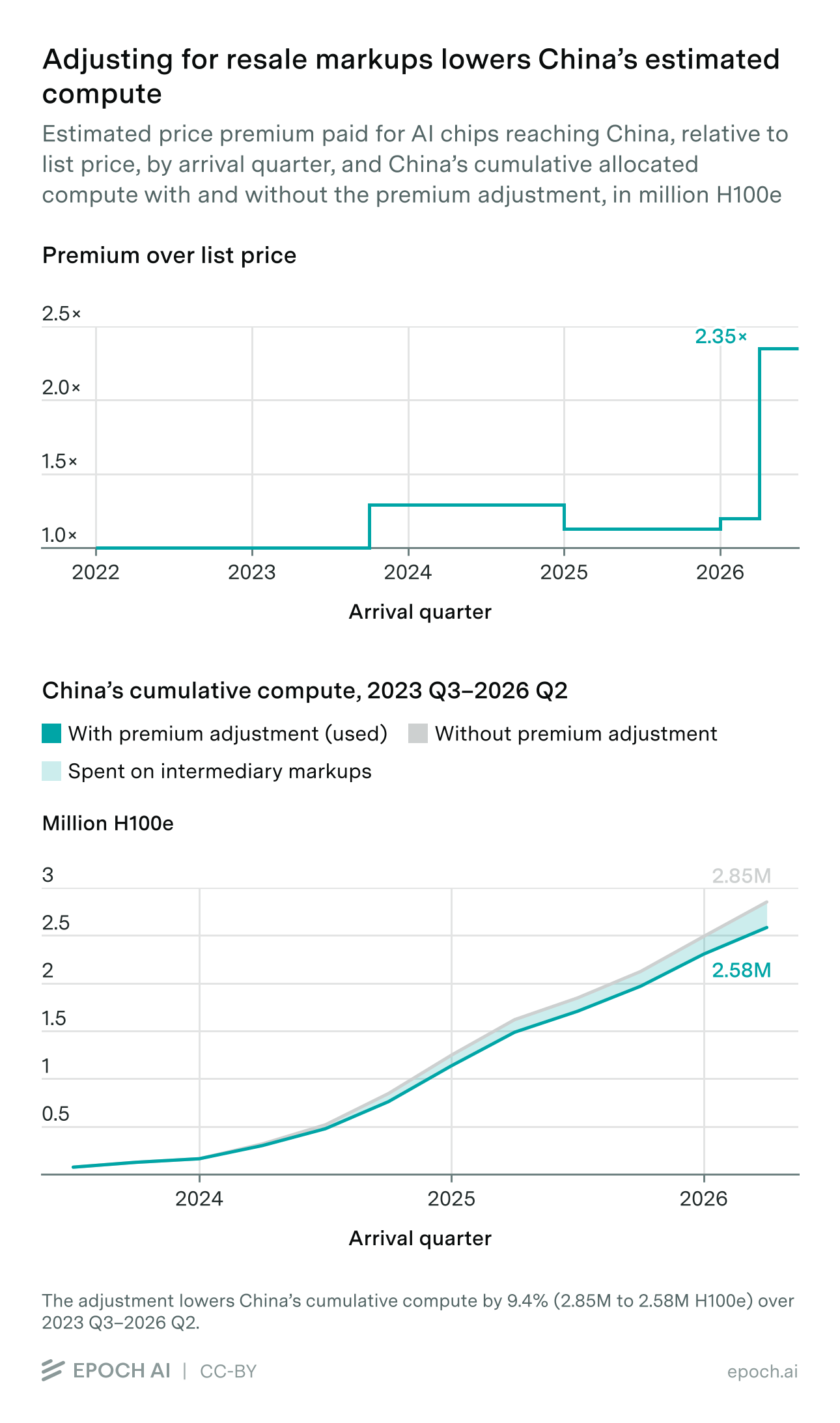
Hardware reaching China after export controls does not change hands at the chip sales list price: an intermediary margin sits between what the customs record shows and what the designer originally charged. Converting China’s customs dollars into units at list prices would therefore overstate its chip count, so we adjust China’s global-pool dollar allocation for the estimated premium before converting it to units. The dated premium applies to the customs-dollar budget for the arrival quarter before allocation to eligible merchant models. Its effect depends on both customs geography and the sales budget interpolated into that quarter.
The premium is a dated series based on reports of diverted-chip sales, benchmarked against the per-model prices in chip sales:
| From | Premium | Basis |
|---|---|---|
| 2022Q1 | 1.00× | Standard A100/H100 sales to China still lawful (the October 2022 controls phased in through 2023); legal trade carries no diversion margin |
| 2023Q4 | 1.29× | 8-GPU Hopper servers through 2024: four observations at +23–35% |
| 2025Q1 | 1.13× | Hopper servers +6%, a B200 rack +20% |
| 2026Q1 | 1.20× | A bundled 8×H200 server at +19.7% |
| 2026Q2 | 2.35× | Active enforcement: B300 +116% and DGX B300 +147%, post-crackdown |
4.4 Results: AI chip arrivals by country
Cumulative allocated arrivals through June 2026 total 27.391 million H100-equivalents and 24.184 million AI chips. These estimates use the 2021 reference, historical warm-up, retrospective charge-backs, monthly chip content and fixed calendar customs quarters. The primary estimate reflects the adopted assumptions; it is not a simulation median. The table uses the October 15, 2026 allocation and its matching provisional 144-case pilot, reporting primary estimates, conditional 90% intervals and structural envelopes (Section 4.5), with compute in millions of H100-equivalents. The primary estimate need not be at the midpoint of the structural envelope, which spans alternative assumptions without assigning them probabilities.
| Destination | Primary estimate, M H100e | Conditional 90% | Structural envelope | Share |
|---|---|---|---|---|
| United States | 19.764 | 17.47–21.83 | 14.17–24.96 | 72.16% |
| China | 2.637 | 2.26–2.96 | 1.90–4.19 | 9.63% |
| European Union | 1.388 | 1.24–1.58 | 1.03–2.57 | 5.07% |
| Malaysia | 0.668 | 0.59–0.76 | 0.49–1.49 | 2.44% |
| India | 0.442 | 0.40–0.50 | 0.30–0.72 | 1.61% |
| Japan | 0.432 | 0.37–0.49 | 0.19–0.56 | 1.58% |
| Australia | 0.386 | 0.34–0.44 | 0.20–0.57 | 1.41% |
| United Kingdom | 0.340 | 0.30–0.38 | 0.22–0.50 | 1.24% |
| Indonesia | 0.219 | 0.20–0.25 | 0.18–0.33 | 0.80% |
| South Korea | 0.105 | 0.09–0.13 | 0.04–0.94 | 0.38% |
| All others | 1.009 | 0.89–1.16 | 0.82–1.53 | 3.68% |
The US receives 66.8% of allocated units and 72.2% of compute; China receives 18.2% and 9.6%, respectively. South Korea’s primary estimate is 0.105 million H100e. Country uncertainty endpoints cannot be summed: shares are normalized within each draw, and “All others” is summed within each draw before its percentiles are computed.
Known weaknesses
- Within the eligible pools, country allocations inherit the model’s proportional mix rather than observing each destination’s actual purchases. A country unusually concentrated in one model can therefore have a different true unit-to-dollar and compute-to-dollar conversion. The probability model does not comprehensively cover this country-specific mix error.
- The uniform monthly interpolation cannot capture sales concentrated near quarter-end or differences in shipping delays across countries. These assumptions affect the arrival budget as well as its geographical allocation. The uncertainty scenarios hold this timing convention fixed and do not measure variation in shipment-to-sale delays.
- Sixteen destinations are measured from their own customs records: the US, China, Hong Kong, the EU, South Korea, Malaysia, Singapore, the UK, Japan, Indonesia, India, Thailand, Mexico, and, on their Comtrade submissions, Saudi Arabia, Australia and Canada. Other destinations depend on selected exporters’ declarations. Their estimates can miss shipments from excluded exporters, include overlapping declarations, or count hardware that later moves elsewhere. The primary estimate assumes inferred arrivals remain locally; customs evidence does not establish that assumption.
- China’s price premiums are rough estimates, and they affect its GPU numbers considerably.
- These stocks do not deduct subsequent relocation or retirement; Section 6 discusses the resulting limitations.
4.5 How uncertain the estimates are
Our estimates can be wrong in two ways. The inputs can be off: sales volumes, prices and imported-content shares. And we can misread what the trade contains: expensive memory can look like accelerator boards, and an average server price can hide very different products.
We report two ranges. The 90% interval varies the inputs under our main assumptions. The structural range repeats this across 144 alternative sets of assumptions about trade content, the baseline and server product mix, and runs from the lowest 5th percentile to the highest 95th percentile across them. We don’t assign probabilities to the alternatives, so the structural range is not a 90% interval, and it only covers the alternatives we tested.
Each draw varies the indexed reference, imported content of exports (k), physical-classification thresholds, selected chip-content fractions and global sales inputs. We recompute trade netting, baseline weights, quarterly offsets, retrospective charge-backs, chip content and country allocation. The adopted model uses the 2021 reference without an AI carve; one structural alternative restores the 2022 reference with its carve. Sales are sampled in their original reported quarters before interpolation into arrival quarters.
Parameter draws vary around the values used for each case. Baseline and k errors combine shared and country-specific components that persist across quarters; classifier thresholds and category-content shifts also persist. National tariff classifications retain precedence, and import-derived k follows the content model rather than receiving a second independent k shock. On rows covered by an explicit server-mixture model, the mixture replaces the additive server-content shift. Appendix A gives the priors and structural cases.
Our chip sales estimates include uncertainty ranges for each model’s sales, but those ranges do not specify how errors move together across models or quarters. We assume that an overestimate of one model’s sales tends to persist across quarters, and that models from the same designer share some uncertainty. We fit positive two-piece lognormal distributions to the model-level quantity and H100-equivalent quantiles in chip sales. Dependence is introduced through a shared designer component, with a correlation of 0.5 between the underlying Gaussian variables. This is an assumption of this project about joint uncertainty, not an estimate taken from our chip sales data; Appendix A.2 gives the construction.
Price and quantity uncertainty are connected. If hardware revenue is $1 billion, a price of $25,000 implies 40,000 chips, while $20,000 implies 50,000. Those quantity estimates represent different prices for the same spending. Drawing price and quantity independently would also generate combinations inconsistent with that revenue estimate.
For Nvidia, we therefore draw quantity and recover the corresponding price using a shared hardware-revenue factor informed by our chip sales notebook. For AMD, Google and Cambricon, we assume that a higher quantity reflects both lower prices and higher spending, dividing the change equally on a logarithmic scale. That split is our modelling judgement. Designers with direct-volume estimates receive a separate illustrative price prior. Appendix A.3 specifies the equations and alternatives.
Each of the 144 cases uses the same 64 proposals: 32 from each of two independently scrambled Sobol sequences, giving 9,216 case–draw combinations. All passed the warning-based acceptance filter, so filtered and unfiltered endpoints coincide. Each draw conserves its own global units and H100-equivalent supply. These checks establish internal consistency, not the validity of the priors or product interpretations.
Through June 2026, the world primary estimate is 27.39 million H100e, with a conditional p5–p95 interval of 24.64–30.21 million. The structural envelope has the same world endpoints because every case allocates the same sampled global arrival budget.
With 64 proposals per case, each 5% tail is informed by roughly three draws. The maximum half-to-full endpoint movement is 8.13%, and the maximum gap between the two independent scrambles is 15.95%. These results remain a provisional small-sample pilot, not a convergence-certified release. The diagnostics measure numerical stability, not the validity of the priors or whether the model covers the true uncertainty; broad comparisons are more reliable than precise endpoints.
The structural cases vary ambiguous parts and other-unit content, the baseline index, server product mixtures and which products remain after baseline subtraction. They also include a combined low-content case, the 2022 reference and a high-China case that removes the diversion premium and excludes Vietnam from China’s boards reference. The 48 content, reference and selection specifications include an isolated merchant-only classifier-price alternative; crossing each with 0%, 50% and 100% Malaysia server-gap deductions gives 144 cases. No probabilities are assigned to these structural choices. All retain monthly content and the two-month sales-to-arrival convention. Reporting errors, country-specific model mixes, premiums and shipment timing are not comprehensively covered.
For missing exporter physical fields, low and high imputation scenarios use donor-content percentiles, expanded where necessary to include the mean used by the primary estimate. These are alternative content assumptions, not confidence bounds. Separate retention scenarios test the possibility that inferred arrivals move onward: capacity not retained locally is reported as unlocated rather than reassigned to a guessed destination. These scenarios preserve global supply and carry no assigned probabilities. They remain separate from the 144 cases used for the reported envelope.
5. How reliable the customs records are
Every flow in our dataset should be recorded twice. The exporter’s customs agency records it on the way out, and the importer’s records it on the way in. A mirror check compares the exporter’s and importer’s declarations for the same flow to assess their consistency.
This section runs that check across the whole collection. It reports how often the two sides agree, explains why they so often do not, and shows how much of the disagreement can be reconciled. It then looks closely at Taiwan, whose customs records no international source can verify, and compares our data against BACI, the standard reconciled trade dataset.
The estimator does not use the reconciled mirror values. The mirror analysis suggests three practices: compare economically coherent code families, use physical fields to diagnose value gaps where their definitions and quality permit, and distinguish declared export destinations from final arrivals. Piece counts are not universally more reliable: they can mix modules with systems and can disagree materially across reporters.
5.1 Comparing exporter and importer records
For every pair of countries where we hold both sides, and for each of the nine codes in the basket, we compare A’s declared exports to B against B’s declared imports from A, month by month. That gives 1,190 directed country pairs and about 10,400 combinations of pair and code. Together they cover roughly $6 trillion of trade that both sides recorded over 2022–2026. A perfect mirror is a ratio of 1.00. We count anything within ±20% as agreement, which is about the room that freight, insurance and currency conversion should need.
The two countries’ records rarely agree. Only 18% of the combinations land within ±20%, and the median disagreement is a factor of 2.3.
Three facts narrow down what that disagreement is. It is not a bias in one direction: the median ratio is 0.88, close to 1, so importers as a group are not reporting systematically more or less than exporters. It is not a calendar effect either. Scored monthly, annually, or pooled over the whole window, the agreement rate stays at 18–20%, and if shipments were simply straddling a month or year boundary then pooling would fix it. And it is mostly not about pricing. In 89% of the disagreeing corridors that report weight on both sides, the two countries disagree on the tonnage as well, and freight and insurance move value rather than kilograms. That leaves pricing able to explain at most about a tenth of the flagged corridors.
Pricing differences alone cannot explain these discrepancies. Differences in coverage, commodity classification and partner attribution also matter. We examine three mechanisms behind these discrepancies. Section 2.6 introduced the first two: countries file the same hardware under different codes, and exporters record where a shipment was sent while importers record where it was made.
The third mechanism is the largest, and it belongs to the re-export hubs. A hub records goods leaving for a partner, but the partner does not record them as arriving from the hub. It records them as arriving from wherever they were made, so the hub’s export appears nowhere in the partner’s customs records. Hong Kong reports $323 billion of processor re-exports (8542.31) to mainland China over the window, and China books almost none of it as coming from Hong Kong: it books those chips as arriving from Taiwan and Korea, where they were made. Across the collection, 823 combinations of pair and code are one-sided in this way, with one country recording a flow that the other records nothing of.
5.2 How much of the disagreement we can explain
Each mechanism has its own fix, and because the mechanisms are different, the fixes add up rather than overlap. We apply them in order. Each one is scored the same way: what share of the trade dollars now sits in corridors where the two countries’ records agree within ±20%? We score dollars rather than corridor counts, because a fix aimed at the largest flows should be judged on the largest flows.
- Record both sides by where the goods were made. The importer side already is, since customs books imports by origin. The exporter side takes two moves. Five of our sources separate goods a country made itself from goods it is only passing on: the US, Hong Kong, Singapore, Malaysia, and Canada. Where that split exists, we stop crediting the hub with goods it did not make. Then we credit each hub’s re-exports back to the countries the goods came from, in proportion to what the hub itself imported under the same code. That proportion is an assumption, so we tested it on the largest hub: Hong Kong re-exports goods in almost exactly the origin mix in which it imports them, with a correlation of 0.999.
- Compare families of codes, not single codes. Grouping the nine codes into five families (servers and boards together, logic chips, memory, networking, storage) cancels the classification disagreement inside each family, because both sides are then added up over the same set of codes. The grouping has to be chosen with care. The biggest single disagreement is Taiwan filing servers under 8471.80 that the US books as parts under 8473.30, and those two codes sit under different four-digit parents, so aggregating to four digits cannot cancel it. The family has to span both parents. Coarser grouping also always scores better for a trivial reason, because fewer and larger buckets average out noise. To check that ours wins on economic sense rather than on arithmetic, we scored it against all 1,260 possible regroupings of the same shape. It comes out at the 99.8th percentile.
- Where the invoices still disagree, ask about the goods instead. Any remaining failing corridor whose sources publish piece counts on both sides can be split exactly into a quantity and a unit price. That separates two questions: did the two agencies disagree about what moved, or only about what it was worth? Where the goods can be counted, about two-thirds of the failing dollars fail mainly on price rather than on quantity.
The first step closes the widest gaps in the dataset. Taiwan’s bare-processor exports to China disagreed by a factor of 48, because about $161 billion of them physically travel through Hong Kong and Singapore. Credited to the Taiwan-to-China corridor, that disagreement falls to 2.2×. US servers to Mexico go from 0.12× to 1.4×, and Singapore to Taiwan from 0.04× to 1.1×.
The clearest example of the third step is also the largest failing corridor in the dataset. Taiwan and Hong Kong disagree by 1.7× on the dollar value of the logic chips moving between them, while their piece counts agree to within 1%: 163 billion units against 165 billion.
| Step | Share of trade $ where the two countries’ records agree |
|---|---|
| Raw mirror, code by code | 24% |
| + origin re-attribution | 36% |
| + code families | 57% |
| + goods agree even where invoices don’t | 66% |
The price gap exposed by this diagnostic is persistent. Taiwan-made chips are booked into Hong Kong and Singapore at 1.5 to 2.2 times Taiwan’s declared values across the historical sample, including before the AI boom. Related-company invoicing is a plausible explanation: the two declarations may value different transactions in the same supply chain. Where comparable piece counts agree, they help distinguish valuation gaps from quantity gaps. This does not establish that physical fields are accurate on other corridors or that quantities can identify accelerator content by themselves.
Some remaining discrepancies cannot be investigated because piece counts are missing; others remain unexplained despite the available physical data. Nearly half of the unreconciled dollars cannot be diagnosed at all, because one side publishes no usable piece counts. Korea publishes none, which is the highest-value data gap left in the project. Most of the rest is the pricing gap just described. Corridors where the two countries still appear to disagree about physical goods, after every correction, hold about 6% of the trade we can check from both sides; this is the same trade the chart below shows as the 14.5% of unreconciled value that is unexplained. The largest of them is Korea’s memory exports to Taiwan, which Section 5.3 returns to.
To check for errors in our collection or processing, we repeated the comparison using UN Comtrade and separate code. Comtrade reproduces the aggregate agreement rate, at 17–18% against our 18–20%, and it reproduces the individual corridor gaps, with a correlation of 0.88 in logs. Customs mirrors disagreeing by a factor of two is a general property of trade statistics, not something our basket or our processing introduced.
One difference is specific to our basket, though. We also ran a control basket of nine ordinary goods: cars, packaged medicines, t-shirts, coffee, furniture, footwear, toys, plastic bottles and aluminium. For ordinary goods the largest flows mirror well, so 45% of their trade dollars agree within ±20%. For chips only 25% do. Ordinary goods disagree in their small flows, and chips disagree in their biggest ones, because the biggest chip flows are the hub-routed, related-company ones.
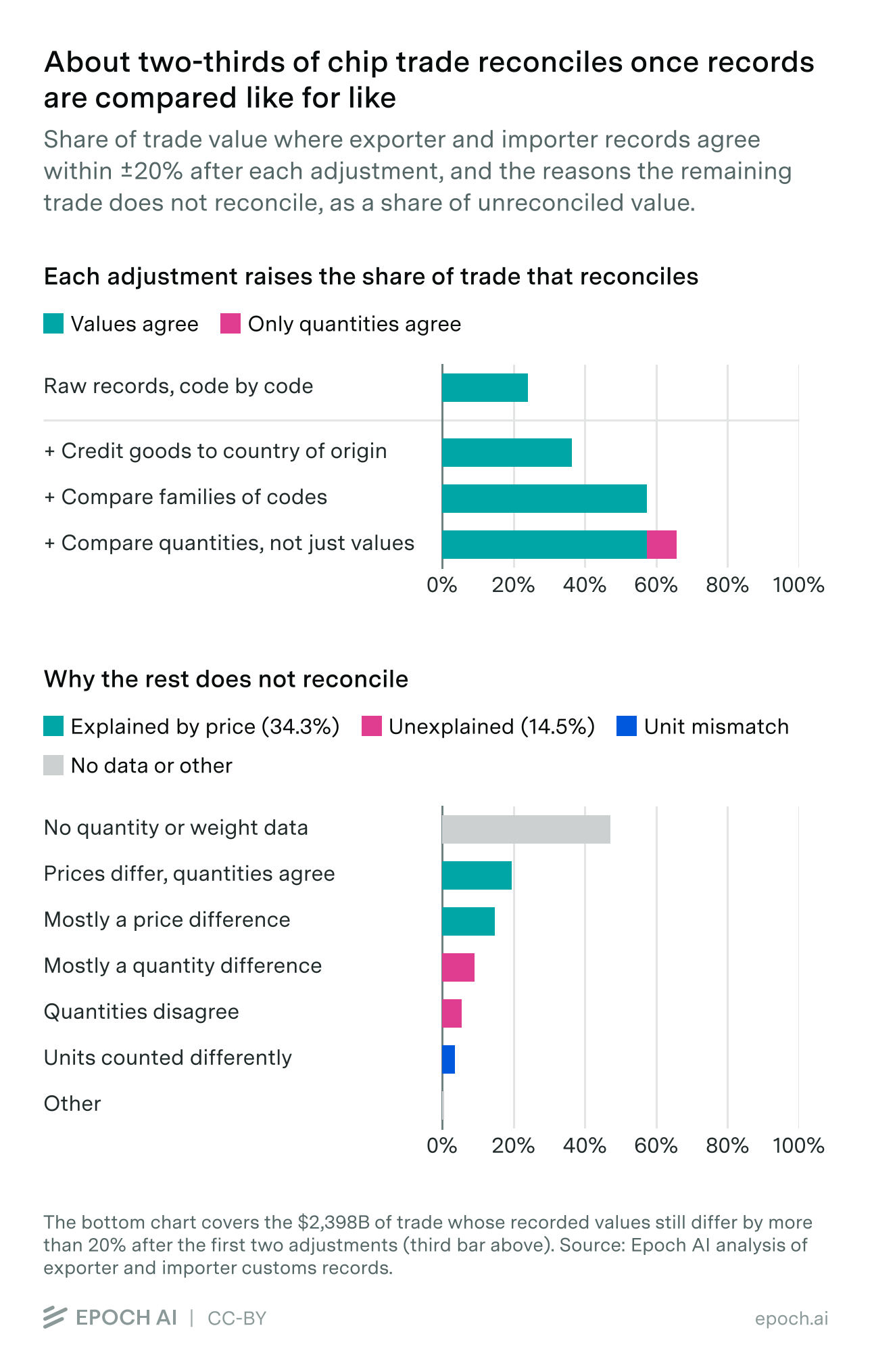
5.3 Taiwan’s customs records
Taiwan gets a closer look for three reasons. It is where essentially every advanced accelerator is made, so its export dataset is the one record of everything that later arrives somewhere, and the manufacturing-side check the destination estimate is compared against (Section 3.5). It is also the one major reporter that no international dataset can check, because Taiwan is not a UN member and does not report to Comtrade, so global datasets carry it only as a residual rebuilt from its partners’ declarations. And it sits on more of the remaining disagreement than any other country, with $2.3 trillion of checkable trade and six of the ten largest unresolved corridor gaps.
As a source it is among the best we hold, as Section 2.5 showed: the fastest publisher in the collection at 7–10 days after month end, net weight on all of its value, piece counts on about a third, and 11-digit national detail. Its tariff tree carves out no AI-specific lines, so all of this hardware rides the standard six-digit codes.
Taiwan’s declarations agree with partner records more often than the collection average. Weighted by dollars, 83% of Taiwan’s trade either mirrors outright (60%) or fails only on the related-company price gap while the goods themselves agree (23%). The comparable figure for the collection as a whole is 66%, and only 6% of Taiwan’s trade is genuinely unexplained. Its export side is the stronger half at 89% reconciled, and its memory exports reconcile at 94% on value alone, with no pricing story needed.
Taiwan’s use of 8471.80 accounts for a large share of its code-level disagreement with importers. It files roughly half of its basket exports under 8471.80, “other ADP units”, a code most importers barely use. That is the single largest code disagreement in the dataset, and it is why comparing Taiwan’s flows one code at a time misleads. Against the US, the individual codes range from 0.18× to 2.90×, while the family total agrees to within 4%.
| HS-6, Taiwan → US, 2022 – early 2026 | Taiwan records | US records | Ratio |
|---|---|---|---|
| 8471.50 processing units | $94.3B | $140.3B | 1.49× |
| 8471.80 other ADP units | $160.8B | $29.2B | 0.18× |
| 8471.49 systems | $3.4B | $5.7B | 1.68× |
| 8473.30 parts | $37.2B | $108.1B | 2.90× |
| 8471 + 8473 family | $295.7B | $283.2B | 0.96× |
Taiwan’s declared export destinations are weaker evidence of final location than of departure. The destination known at export can differ from the country where the hardware eventually remains. The estimator therefore prefers destination import records where available. Elsewhere it uses selected exporters’ declarations, including Taiwan’s. These estimates have weaker coverage and cannot establish local retention. They may also contain overlapping declarations when an original exporter names the final destination and an intermediary reports the same shipment as a re-export.
Korea’s memory exports to Taiwan (8542.32), which include HBM used in accelerators, remain unreconciled after these adjustments. That corridor disagrees by 1.32× on value and by 2.14× on weight, and those two point in opposite directions from every other memory corridor we hold. It is the only large corridor in the project where the physical evidence itself disagrees. Taiwan’s imported-memory line reconciles at just 6%, with more than half genuinely unexplained. Korea publishes no piece counts, so we cannot yet separate a weight-convention artifact from real under-declaration. Comparable Korean piece counts would help distinguish these explanations.
5.4 Why we do not use BACI’s reconciled data
Section 2.2 explained why raw Comtrade cannot answer this project’s question. The obvious next candidate is BACI, CEPII’s reconciled trade database, which is built on Comtrade and is the standard dataset in empirical trade research.
BACI addresses exactly the problem this section measures. Where two countries declare the same flow differently, it produces one number: it removes estimated freight and insurance from the import side, scores each country’s reporting reliability against all of its partners, and publishes a single value per exporter, importer, product and year. Because we hold both raw declarations, we can watch that reconciliation work on our own basket. We joined BACI’s current release (HS22, version 202601) to our data for 2022 to 2024, which is about 26,000 combinations of corridor, code and year, and $3.5 trillion of trade.
On the basket as a whole, BACI is a reasonable compromise between the two countries’ records. Its value falls between the two national declarations on 75% of the joined dollars. It tracks the importer’s figure more closely than the exporter’s, landing within ±20% of the importer on 53% of dollars against 39% for the exporter, which is a sensible default because imports are the better-policed direction.
On the corridors this methodology relies on, the two countries’ records differ for the structural reasons of Sections 5.1 and 5.2, and averaging them produces a figure that matches neither the shipping record nor the origin record.
| Corridor, 2022–2024 | Exporter records | Importer records | BACI |
|---|---|---|---|
| Taiwan → US, 8471.50 | $26.7B | $28.3B | $28.3B |
| Taiwan → US, 8471.80 | $45.2B | $12.3B | $12.4B |
| Taiwan → US, 8473.30 | $19.7B | $48.4B | $22.9B |
| Taiwan → US, 8471 + 8473 family | $94.6B | $91.0B | $65.9B |
| Taiwan → China, 8542.31 | $5.1B | $243.3B | $90.8B |
| Hong Kong → China, 8542.31 | $205.2B | $0.03B | $0.03B |
| Korea → Taiwan, 8542.32 | $21.5B | $35.8B | $26.5B |
The table illustrates three limitations. First, reconciling individual codes can understate trade when countries classify the same goods differently. BACI reconciles one product code at a time. That works when both countries file the same goods under the same code. Taiwan and the US do not: Taiwan puts servers under 8471.80 that the US books as parts under 8473.30. So on each of those codes BACI has to choose between two figures that are far apart, and on both it lands near the smaller one: $12 billion where Taiwan declared $45 billion, and $23 billion where the US booked $48 billion. Adding its codes back up gives $65.9 billion for the server-and-parts family, against $94.6 billion in Taiwan’s records and $91.0 billion in the US’s. The reconciled number comes out below both of the numbers it was reconciling.
The same pattern appears on other corridors. We checked it across every corridor where the two countries agree at family level, which is the closest thing to ground truth this data offers. BACI recovers 94% of the agreed value overall and 86% on servers and boards, with about a fifth of the agreed dollars landing more than 20% below both countries’ records.
The second is what happens to hub flows. BACI correctly refuses to credit Hong Kong with $205 billion of re-exported processors, adopting China’s near-zero instead. But the goods do not fully reappear where they came from. For Taiwan to China it averages the $243 billion of Taiwan-made arrivals that China booked against the $5 billion Taiwan declared sending directly, and lands at $91 billion, which is 63% below what China’s customs actually recorded arriving. Most of the re-exported value goes missing rather than moving to the right corridor. We keep the two declarations apart instead, and credit hub flows using the hubs’ own re-export data.
The third is what happens where the two countries genuinely disagree about goods. On the Korea-to-Taiwan memory corridor in the last row, BACI splits the difference on a disagreement whose cause is still unresolved on physical evidence (Section 5.3). The available evidence cannot validate the reconciled figure.
BACI reconstructs Taiwan’s trade from partner declarations. BACI has no Taiwan reporter, so its code 490, “Other Asia, not elsewhere specified”, is rebuilt from what Taiwan’s partners declare, and CEPII’s own FAQ recommends it as a Taiwan proxy. On this basket the import side of that proxy holds up well, at 0.96 times Taiwan’s own customs records. The export side is the one that matters for AI hardware, and it runs at 1.31 times Taiwan’s own declarations, with a median corridor discrepancy of 1.48× and only 40% of dollars within ±20%. The reconstruction inherits its partners’ view of Taiwan’s exports.
In a historical test using the earlier quarterly-content estimator, averaging importer and exporter declarations cut China’s customs dollars so far that they could no longer cover the China-specific chips that chip sales records as lawfully sold there; the typical-quarter match fell from 1.03 to 0.86. Current measured-country flows therefore retain the destination’s own records. The exceptions are the UK’s reconstructed 2021 EU-import history and associated indices, and the 50% Malaysia server-gap deduction (Section 3.2). These are targeted adjustments rather than a general averaging of importer and exporter declarations.
The last limitation is timing. BACI is annual and comes out each January. Version 202601 is the first to include 2024, and CEPII warns that the newest year is revised substantially in the following release. In the earlier quarterly-content diagnostic, 74% of customs-derived chip dollars over 2023Q3–2026Q1, about $240 billion of $325 billion, arrived in quarters after December 2024. None of that is in BACI yet, and it will not be until 2027.
Known weaknesses
- The mirror check only covers pairs where we hold both countries. It validates the corridors this methodology uses, not world trade. Corridors touching countries we do not hold, such as Vietnam and the UAE, still rest on one side only.
- The ±20% agreement band is a convention. We report results by corridor count and by dollar share, and no conclusion here changes if the band is widened: ±30% raises the share of corridors that match to 64% and ±50% to 75%.
- Splitting a disagreement into quantity and price needs piece counts from both sides, and those exist for only about half of the failing dollars. Korea publishes none at all, which is also why the Korea-to-Taiwan memory anomaly stays open. Its Comtrade mirror does carry piece counts, so this is a known fix we have not built.
- A piece count has its own ambiguity, because a die, a module and a finished system all count as one piece. Corridors where the quantity gap and the price gap point in opposite directions are flagged as counting problems rather than treated as resolved.
- The BACI comparison runs on BACI’s terms: annual, six-digit, and with its 2024 still provisional. Its code 490 is a residual group that is mostly but not exactly Taiwan. We compare against our raw declared values, including re-exports, which is what BACI takes from Comtrade.
6. Limitations and next steps
Chip content is the weakest step. Declared value per unit and per kilogram can’t reliably separate accelerator boards from standalone memory, ordinary computer parts or assembled systems. Where countries label memory modules in their tariff codes, we exclude them, and the structural cases test other readings of ambiguous trade, but not every possibility. Our central estimate assumes the excess above the baseline has the same product mix as the overall flow.
Customs data can also simply be wrong. Misclassification, valuation errors, omitted shipments, concealed destinations or falsified declarations can produce systematic errors that neither more simulation draws nor a narrower parameter prior will resolve. Agreement between mirror records is useful evidence, but is not proof of correctness when both sides reflect the same transaction records or common reporting practices. The reported intervals do not quantify uncertainty from incorrect customs declarations.
Country allocations depend on model eligibility and a proportional mix within eligible pools; they do not observe every destination’s purchases. Retained cross-border hardware is a proxy for deployment, rather than verified installed or operating capacity. The estimates do not fully account for domestic production outside the observed trade network, later relocation, retirement or changes in shipment-to-sale timing. Recent quarters can be revised by charge-backs and customs updates. China’s intermediary premiums and other source-specific biases are not fully represented by the primary priors.
The baseline rests on assumptions. It assumes AI chip trade in 2021 was negligible and that our indices track ordinary trade afterwards. For the UK, it also depends on reconstructing 2021 imports from the EU.
Exporter-based destination estimates face separate uncertainties about product content, duplicate declarations and local retention. Imputing missing physical fields from observed shipments addresses missing measurements, but does not establish the products in an ambiguous shipment or its final location.
Taiwan and Hong Kong declarations could overlap where Taiwan records the final destination and Hong Kong records the same goods as a re-export. Excluding measured hubs from Taiwan’s residual allocation prevents one form of double counting, but does not establish that all remaining destination flows are distinct. We have not quantified this possible overlap.
Next steps. The most useful check would be dated evidence of where chips are actually deployed: company disclosures of data center locations and chip counts, confirmed deliveries, and credible reports on specific facilities. These need to match on country, chip model and time period, and announced orders should be kept separate from delivered systems. Even partial coverage could show where our estimates go wrong.
We also plan to:
- look for direct evidence of what ambiguous parts and “other unit” imports contain
- test the boards baseline on held-out periods
- check the UK reconstruction
- measure how the estimates change when customs agencies revise their data
Appendices
Appendix A: Probability model and priors
The reference probability model is documented below so that the 90% intervals can be reproduced and challenged. The repository’s uncertainty guide describes the current implementation, how to run it, and how to interpret its outputs and numerical convergence diagnostics. Distribution endpoints listed for triangular priors are supports, not 5th and 95th percentiles.
A.1 Parameter priors
Let \(T\) denote a symmetric triangular variate with support \([-1, 1]\) and mode 0. Each shared or local variate is drawn independently unless a dependency is specified. The resulting parameter is held constant over time within a draw.
Non-AI baseline: multiply the indexed reference constructed from 2021 trade for reporting country or bloc \(c\) by
\[1 + 0.10\,\left(0.70\, T_{\text{shared}} + 0.30\, T_c\right)\]The shared multiplier applies where no country-specific setting exists. The weighted sum of triangular shocks is not itself triangular; 70/30 are amplitude weights, not variance shares or a correlation coefficient. These perturbations apply from January 2023. The headline uses the 2021 reference with no AI carve; the 2022-reference alternative retains its own carve.
Export k: add \(0.10\,\left(0.70\, K_{\text{shared}} + 0.30\, K_c\right)\) and clip the result to \([0, 1]\). This applies to k inferred from gross export physical evidence and its fallback pooled across its export records. Import-derived k inherits the perturbed import content and receives no additional independent k shift. K shocks are independent of baseline shocks before feasibility conditioning.
Physical classifiers: multiply the unit-price thresholds by a global triangular factor with minimum 0.75, mode 1 and maximum 1.25; draw a separate factor with the same distribution for the density thresholds. Gross observed quantities and weights are unchanged. Selected physically classified 847150 and 847330 contents receive separate category shifts with triangular support \([-0.10, 0.10]\) and mode 0, clipped to \([0.05, 0.93]\). Classifications based on national tariff codes retain precedence. Where an explicit server-mixture model is applicable, sampled chip prices and the price-anchor factor enter its system-price calculation; the additive server-category shift is not applied to those same rows.
A.2 Sales marginals and correlation
For a source median \(Q_{50}\) and quantiles \(Q_5\) and \(Q_{95}\), draw a standard normal latent variable \(z\) and set
\[Q = \begin{cases} Q_{50}\, e^{\sigma_- z} & z < 0 \\ Q_{50}\, e^{\sigma_+ z} & z \ge 0 \end{cases} \qquad \sigma_- = \frac{\ln(Q_{50}/Q_5)}{1.64485}, \quad \sigma_+ = \frac{\ln(Q_{95}/Q_{50})}{1.64485}\]This exactly matches the three valid source quantiles and keeps quantities positive. It does not assume that halving the median and doubling it are equally likely unless the supplied lower and upper log-spreads are equal. Missing or nonpositive bounds fall back to the median; remaining quantiles must be correctly ordered.
For model \(m\) made by designer \(d\),
\[z_m = \sqrt{0.5}\, Z_d + \sqrt{0.5}\, Z_m\]with independent standard normal designer and model components. This gives a 0.5 Pearson correlation between latent Gaussian variables for models from the same designer. The same model rank is used in every quarter and for both its unit and H100e quantile transforms; different designers are independent before conditioning. The assumption represents persistent common uncertainty, and is not a fitted correlation of observed sales.
A.3 Joint price and quantity
Let \(q = Q/Q_{50}\) be the quantity multiplier and \(p = P/P_0\) the price multiplier. For Nvidia, \(p = r/q\), so the expenditure multiplier is \(qp = r\). The common revenue factor \(r\) is lognormal with median 1 and log-standard deviation
\[\sigma_{\ln r} = \frac{\ln(0.99/0.96)}{2 \times 1.28155}\]using the relative uncertainty in the chip sales notebook’s 0.96–0.99 hardware share (an 80% interval). Thus a larger quantity draw generally implies a lower price at nearly unchanged revenue. We construct this relationship from the published inputs of our chip sales data, which do not include the full joint distribution of prices and quantities used here.
For AMD, Google and Cambricon, the reference rule is \(p = q^{-1/2}\), giving expenditure multiplier \(q^{1/2}\). This divides the log-quantity movement equally between price and expenditure. Alternative runs assign all of it to price or allow additional conditional price variation at fixed quantities. For other designers with direct-volume estimates, the illustrative price multiplier is lognormal with median 1, 5th percentile 0.8 and 95th percentile 1.25, drawn independently of the quantity rank. These decomposition and price-prior choices are assumptions of this project.
Each draw propagates its own prices, quantities, H100e values and product mix through the estimator and allocator. Joint sales–price draws are constructed on the original reported sales quarters. Draw-specific units, compute and dollars are then interpolated into arrival quarters using the same two-month shift as the primary estimate. This preserves dependence between neighbouring arrival quarters that share a source sales quarter. Allocated world totals equal each draw’s corresponding arrival budget. Country shares are normalized within a draw, and grouped regions are summed within each draw before quantiles are taken.
A.4 Structural scenarios
These scenarios address uncertainty about what the traded products actually are. A high dollar value per kilogram or per customs item can describe an accelerator board, valuable standalone memory, or an assembly containing substantial non-accelerator hardware. Where national codes do not separate those products, the physical measurements alone cannot identify their accelerator content. The test using national tariff labels illustrates the problem: when explicit Korean memory labels are hidden, the density classifier assigns those memory flows about 91% accelerator content on average.
The parameter priors in A.1 vary thresholds and content scores around a chosen interpretation of the data. They do not adequately test whether that interpretation is wrong: for example, whether a high-density parts flow is mostly memory, or whether the baseline removes mostly ordinary servers. The structural cases impose alternative readings and rerun the model. They carry no assigned probabilities.
The original seven composition choices
Let \(c\) denote the content score after the parameter draw. The transformations below apply to ambiguous cells with \(c > 0.05\) and to applicable unmeasured fallbacks. We leave existing classifications unchanged for country–code combinations classified using national tariff subdivisions, and for cells already assigned low accelerator content. Explicitly identified standalone memory remains at zero.
Baseline: retain the classifier’s scores. This provides the conditional 90% interval around the adopted method and the reference against which the other interpretations are compared.
Low parts: set ambiguous 847330 parts to 0.05. This tests whether flows read as accelerator-rich are instead dominated by memory or other non-target parts. The 5% value is the classifier’s low-content benchmark, not a measured memory share or a strict lower bound.
Mixed parts: replace ambiguous 847330 scores with
\[c' = 0.05 + 0.5\,(c - 0.05)\]This moves the estimate halfway towards the low-content benchmark, testing an intermediate accelerator-content share. It does not assert that half of the physical items are memory.
High parts: set ambiguous 847330 parts to 0.93, the accelerator-board benchmark. This tests the opposite error: whether the baseline classifier understates accelerator content in a board-rich flow. Together, the low, mixed and high cases test how much the results depend on interpreting this broad parts category.
Mixed units: apply the same transformation, \(c' = 0.05 + 0.5\,(c - 0.05)\), to ambiguous 847180 units. This code is particularly important for Taiwan-linked trade and China’s allocation. The scenario tests a lower share of target accelerators within these units; it does not assume that the displaced value is specifically memory.
Joint mixed: apply the mixed transformation to both 847330 and 847180. This checks whether ambiguity in the two categories matters simultaneously, rather than changing only one category at a time.
Assembly units: cap ambiguous 847180 scores at 0.73, the HGX-server benchmark. This tests whether high-scoring units are assemblies containing more host hardware rather than accelerator boards. It is an alternative form-factor interpretation, not a claim that every server or rack has the same content.
The 144-case set
The current set has 144 cases: 48 baseline, content and selection specifications, each crossed with Malaysia server-gap deductions of 0%, 50% and 100%. The central conditional interval uses the adopted specification with a 50% deduction. The 48 specifications comprise the following 47 choices plus an isolated merchant-only classifier-price reference.
Twelve baseline/content cases cross three references with four content treatments. The references are the adopted component index for boards and client-IT index for systems, a client-IT index for boards, and a flat systems reference. Content treatments are the adopted classifier, two explicit server mixtures and mixed parts.
Twenty-seven selection cases cross those three references with a capped server ladder or either server mixture, and with proportional, halfway or ordinary-first selection after baseline subtraction.
Six named cases add combined low content, the 2022 reference with its AI carve, low parts, high parts, mixed units and high China. Combined low content caps server readings, classifies the US NESOI boards line by density and uses a merchant-only price reference. High China removes the diversion premium and excludes Vietnam from China’s boards reference.
Two further cases add jointly mixed parts and units, and the other-unit assembly cap. This is a union of selected alternatives, not a full factorial of every assumption.
In the server-mixture cases, let \(u\) be the observed average system value and \(p_0\) the ordinary-system price, set to either $5,000 or $15,000. An accelerator system is assumed to contain eight chips with chip share \(s = 0.73\), giving system price, inferred item share \(a\) and chip-dollar share:
\[p_A = \frac{8 \times \text{ASP}}{s}, \qquad a = \operatorname{clip}\left(\frac{u - p_0}{p_A - p_0},\, 0,\, 1\right), \qquad \text{chip-dollar share} = \frac{a \, p_A \, s}{u}\]ASP includes the sampled price and price-anchor adjustment. These are assumed product configurations, not configurations identified from customs averages. The existing classifier is retained where the mixture is inapplicable, including nonpositive unit values, \(p_A \le p_0\) or \(u > p_A\).
The selection cases distinguish the composition of retained gross trade from that of the excess after baseline subtraction. Let \(N\) be retained value before subtraction, \(E\) the remaining excess, \(c\) its gross chip fraction and \(s\) the chip-share ceiling. Proportional selection gives \(cE\) chip dollars. Ordinary-first selection gives \(\min(cN, sE)\), preserving as much accelerator content as fits within the remaining value. The halfway case averages the two. These rules apply to measured server codes 847149 and 847150; they do not change every product category or every exporter-inferred flow. The capped ladder uses the eligible system-mix ceiling; the explicit mixtures use 0.73.
The larger case set matters for the results. China’s structural envelope is 1.90–4.19 million H100e, against a conditional interval of 2.26–2.96 million. The EU’s envelope is 1.03–2.57 million, against a conditional interval of 1.24–1.58 million. These ranges show dependence on the tested assumptions without establishing which alternative is correct. The 144-case results remain provisional small-sample pilot estimates.
Structural choices are held fixed over the entire history, while parameter and sales–price draws are shared across cases. The reported envelope spans the lowest case p5 and highest case p95. It does not exhaust baseline, product-mixture or allocation uncertainty, and it leaves some broad national tariff classifications unchanged. Exporter-imputation and onward-retention tests remain separate. More draws can improve numerical precision but cannot identify the products or final destinations hidden in ambiguous trade records.
Appendix B: Memory-code reference
The three module codes in Section 3.4 directly support the content correction inside 847330. The following memory-IC lines provide additional supply-chain diagnostics. They are outside the final-hardware allocation basket; their values are not added to accelerator dollars or mechanically subtracted from ambiguous parts. National definitions and import/export schemes must be kept distinct.
- HS 854232: electronic integrated circuits serving as memories; the international six-digit parent contains several memory technologies and product stages.
- Korea 8542321010 / 8542321020 / 8542321030: DRAM / SRAM / flash memory. Korea 8542321090 is other monolithic memory, and 8542322000 is hybrid memory ICs.
- Korea 8542323000: multichip memory ICs. It is a useful HBM proxy on the Korea–Taiwan corridor, but its legal scope is broader than HBM. Korea 8542324000 identifies multi-component memory ICs (MCOs), a different category.
- Taiwan imports 85423200234: finished DRAM ICs, including the line in which Korean HBM arrivals are recorded; it does not uniquely identify HBM.
- US imports 8542320036: DRAM exceeding 1 Gbit, including HBM without a separate HBM identifier. US exports 8542320023: the export-schedule DRAM subdivision; it is not interchangeable with the import code.
- Hong Kong 85423210: multi-component memory ICs; not an HBM-specific category.
- EU and UK 85423239: monolithic DRAM exceeding 512 Mbit, excluding multichip and multi-component forms. EU/UK 85423211 identifies multi-component memories; 85423219 identifies multichip memories; 85423290 covers other multicombinational forms, including stack DRAMs and modules under its stated exclusions. The appropriate HBM classification between the latter categories remains unresolved.
- Japan exports 854232100: uncased memory ICs, including wafers and bare die across memory types. Japan exports 854232921: packaged flash memory. These identify different stages, not interchangeable module flows.
- Japan imports 854232011 / 854232021: monolithic DRAM within the respective unmounted/mounted branches; 854232019 / 854232029 are the corresponding other-memory residuals. The residuals do not isolate stacked DRAM or HBM. Japan has no dedicated multichip/HBM statistical line in the collected schemes.
China’s collected 847330 data provide no equivalent dedicated memory-module split, and Indonesia’s collected 854232 data add no useful detail below the six-digit parent. A missing split is a limitation of identification, not evidence that a flow contains no memory.