We have updated the modeling behind the Epoch Capabilities Index (ECI), which measures and tracks AI model capability using benchmark results. The primary motivation is to provide better-justified uncertainty estimates and to let us calculate how likely one model is to be more capable than another.
The new methodology is documented on our website; this post explains how it differs from the previous frequentist approach and what motivates the changes. We first review the basic setup of the ECI and the previous method, then detail the changes in the Bayesian model and present its results. The appendices cover alternative formulations and the evaluation we used to validate our final modeling choices.
How the ECI turns benchmark scores into capability estimates
The ECI is based on Item Response Theory (IRT), a framework originally developed for educational testing that enables comparisons between students even when they took different exams with varying difficulty. Similarly, we have different sets of benchmark scores for AI models that we want to compare. While classical IRT models the binary chance of answering a single question correctly, we adapt it to continuous outcomes by treating a model’s benchmark score as the expected share of questions it gets right. We only use benchmarks that are scored between 0 and 100%. This section establishes the basics of IRT as applied to the ECI and how it informs modeling in both the frequentist and Bayesian models.
We use a version of the four-parameter logistic (4PL) IRT model in which each benchmark’s floor and ceiling are fixed rather than fitted, so only its difficulty and slope are learned. This is equivalent to a two-parameter (2PL) model on rescaled scores. We assume that a model’s performance on every benchmark depends on a single capability dimension. Each benchmark has a difficulty level and a slope, which sets how quickly scores change as models become more capable. Before fitting, we rescale each benchmark’s scores so that random guessing (the floor) maps to 0 and the highest achievable score (the ceiling) maps to 1. Scores below chance are set to 0 and scores above the ceiling to 11.
Following IRT, we predict the score of model m on benchmark b as:
\[\mathrm{predicted\_score}(m,b) = \sigma(\alpha_b[C_m - D_b]) = \frac{1}{1 + e^{-\alpha_b[C_m - D_b]}},\]where
- \(C_m\) is the model capability,
- \(D_b\) is the benchmark difficulty and
- \(\alpha_b\) is the benchmark slope.
The predicted score follows a standard logistic function. It proposes that a model’s performance on a benchmark depends on its capability relative to the benchmark’s difficulty, scaled by the benchmark’s slope.
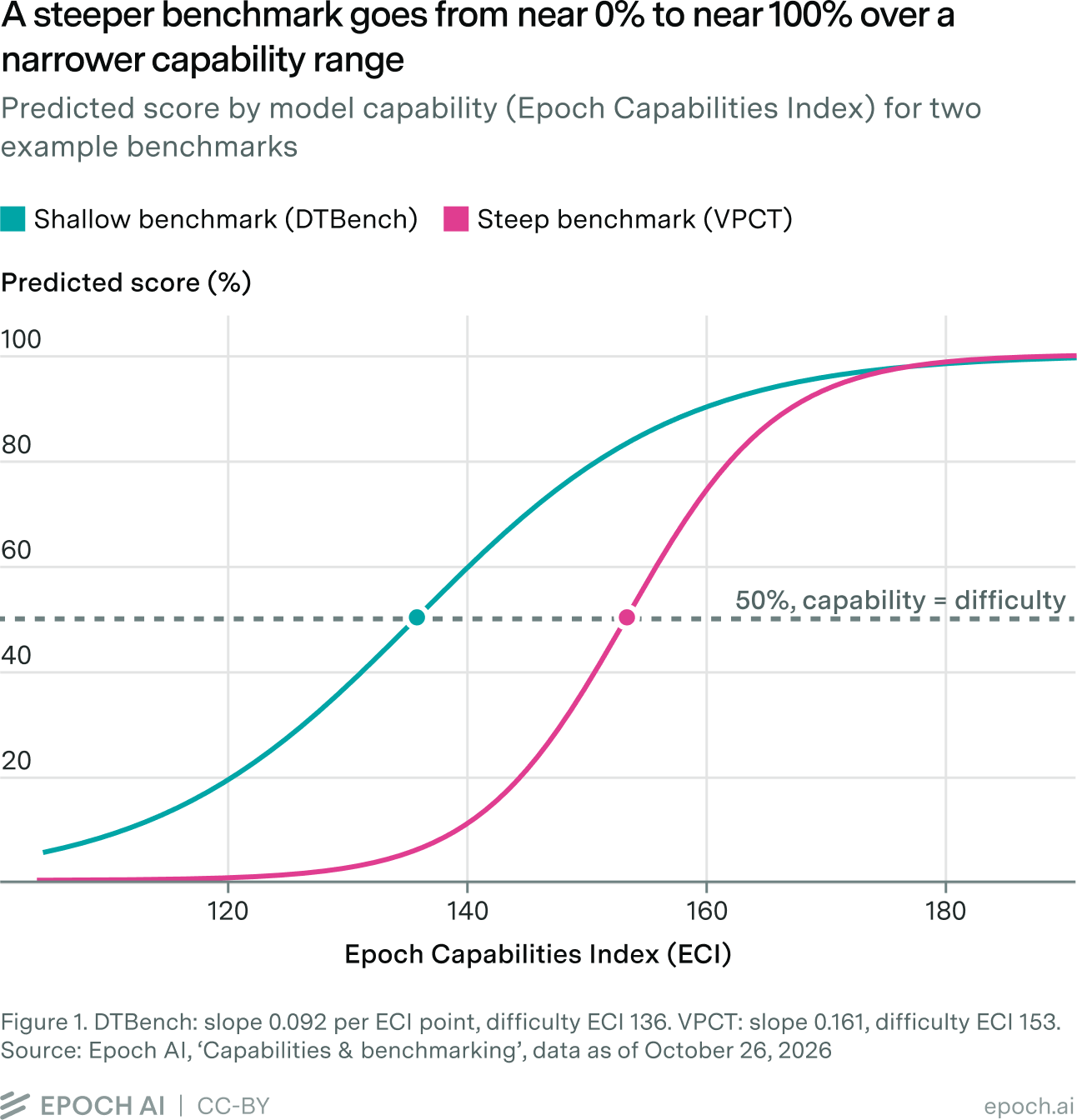
If the model is as capable as the benchmark is difficult, then the predicted score is 50%: \(\mathrm{predicted\_score}(m,b) = \sigma(\alpha_b[0]) = \frac{1}{2}\).
The slope parameter \(\alpha_b\) controls how quickly predicted scores move away from 50% in either direction as the difference between model capability and benchmark difficulty grows (Figure 1).
Our dataset is a set of observed scores, and through our modeling, we fit the three parameters \(C_m\), \(D_b\) and \(\alpha_b\). In the frequentist approach, we seek the parameter values that best explain the observed scores, while in the Bayesian approach we update our probabilistic estimates based on the observed data. For more detail on the data sourcing, see Appendix B.
How the previous frequentist fit worked
Our previous methodology fit the ECI using a frequentist approach, and constructed confidence intervals via bootstrapping. In this section we will explain how this worked in more detail, to give context for our new methodology. Using the frequentist approach, the ECI was calculated by finding the values of \(C_m\), \(D_b\) and \(\alpha_b\) that minimize the squared error of the predicted score against the observed benchmark scores in our dataset. We also included a small regularization term to improve fitting efficiency, which mainly affected very weak models, as we discuss later in the section ‘Frontier ECIs are similar while weak models move down’.
With the predicted score defined as above, the least-squares minimization becomes:
\[\min_{\alpha_b,\, D_b,\, C_m} \sum_{n=1}^{N} \left(\mathrm{predicted\_score}_n - \mathrm{observed\_score}_n\right)^2 + \frac{0.1}{M + 2B - 2}\left(\sum_{b=1}^{B} \left(\alpha_b^2 + D_b^2\right) + \sum_{m=1}^{M} C_m^2\right)\]Here N is the total number of observations we have (one model score on an individual benchmark), B is the total number of benchmarks, and M is the total number of models.
The parameter values were constrained as: \(\alpha_b \in [0.1, 10]\), with the WinoGrande slope fixed at 1 (a benchmark which was selected due to its good coverage of the original benchmarks in the ECI when it was launched). We similarly constrained all \(C_m, D_b \in [-10, 10]\), although none of these constraints are binding and were included only for computational convenience.
After fitting the model on the ‘raw’ parameter scale described above, we applied a linear transformation to fix the location and scale of all parameters, by assigning Claude 3.5 Sonnet an ECI of 130 and GPT-5 an ECI of 150. This gives the ECI a consistent interpretation over time, relative to the two anchor models.
Too few scores per model for bootstrapping to be justified
Our previous methodology estimated uncertainty in the ECI results with bootstrapping, reporting 90% confidence intervals around the point estimate. We aimed to assess how each model’s ECI could have differed if we had observed a slightly different set of benchmark results.
We used 500 bootstrap samples, each holding the set of models fixed and resampling each model’s benchmark results with replacement, keeping its number of observations the same, and refitting the entire model for every sample. Each sample yields slightly different ECI scores, and the 5th and 95th percentiles form the confidence interval bounds.
Each model’s results are resampled independently, with replacement, from its own scores: ten for the median model and as few as four. A bootstrap works when there is enough data for each resample to look like a fresh set of results. On average, each resample leaves out about a third of a model’s scores and counts others more than once. With so few scores per model, this shifts a model’s ECI considerably and the spread across resamples is not a reliable measure of the real uncertainty in its ECI.
What changes in the Bayesian model
The previous frequentist approach had two notable weaknesses: uncertainty via bootstrapping is not justified in such a small data regime as discussed above, and it’s not designed to compare models directly. We chose a Bayesian model to address both points. Bayesian models naturally incorporate uncertainty; the outputs of our model fitting are probability distributions, which means we can take uncertainty estimates directly from this output, including the full observation dataset.
The basic elements of Bayesian modeling are:
- A likelihood, which states how likely we are to observe data given the internal parameters of the model
- Priors, which give our initial expectations for the distributions of those internal parameters
- The posterior, which we obtain by fitting the Bayesian model to our data using the likelihood and priors defined above
Below, we describe in five sections the changes made to the modeling:
- The model fitting: sampling the posterior instead of finding one best fit.
- The likelihood: using a beta likelihood, which keeps all probability between 0% and 100% and lets noise shrink near those limits.
- The noise: letting the model learn that benchmarks vary in how ‘noisy’ their results are.
- The scaling: fixing the scale with the full set of benchmarks, not a single reference benchmark.
- The priors: flat priors on capability and difficulty, shared priors on slopes and noise.
Sampling the posterior instead of finding one best fit
The posterior of a Bayesian model usually cannot be calculated directly, so instead we draw samples from it using Markov Chain Monte Carlo (MCMC)2. Each sample is one plausible set of every model’s capability and every benchmark’s difficulty, slope, and noise. Taken together, the samples approximate the posterior. Instead of selecting a single best-fitting parameter combination, these samples approximate a probability distribution for each model’s ECI. We report the mean of this distribution as the model’s ECI (after per-sample rescaling to set Claude 3.5 Sonnet to 130 and GPT-5 to 150) and its 90% credible intervals3 are precisely the 90% probability mass intervals of this distribution running from the 5th to the 95th percentile.
As all parameters are jointly estimated, we can look at the uncertainty in functions of the ECI, such as the gap in ECI scores between two models, to assess the probability that one is more capable than another. We present an example of this type of gap analysis in the section ‘How likely one model is to be more capable than another’.
The beta likelihood
We have described how the IRT model gives a predicted score for each model on each benchmark. To fit it statistically, we need to measure how well the predicted scores match the observed scores. In Bayesian modeling, this comes from the likelihood: for any set of parameter values, it says how probable each observed score is, given the model’s predicted score.
The previous frequentist methodology, which minimized the squared prediction error, is comparable to a Bayesian model with a normal distribution that has the same noise for every predicted score. When using least-squares minimization, predicting 50% against an observed 55% is penalized just as much as predicting 90% against 95%. However, it seems reasonable to expect the noise to shrink as the predicted score gets close to 0 or 100%. Another issue is that while the predicted score function itself always stays between 0 and 1, a normal likelihood with constant noise assigns probability to scores below 0 and above 1, which is undesirable (Figure 2).
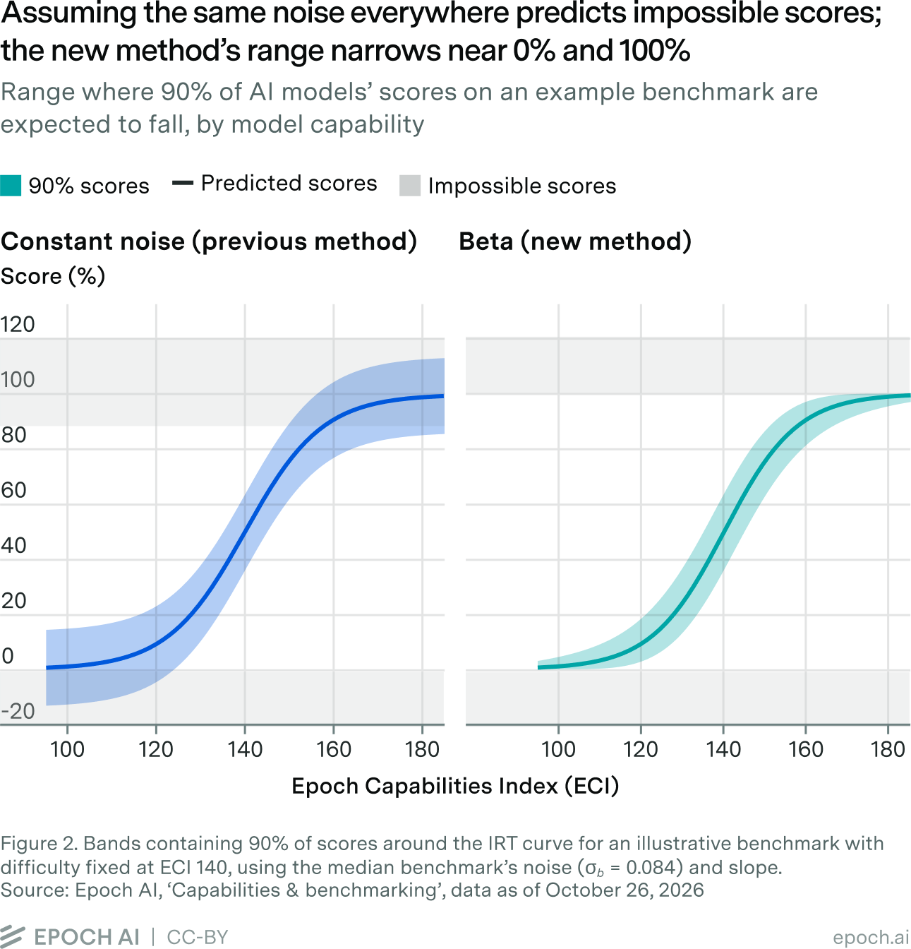
We can replace the normal distribution assumption with a beta distribution for the likelihood function. The beta is a natural choice as it already has support strictly between 0 and 1, and its noise shrinks as scores approach 0 or 14 (Figure 3).
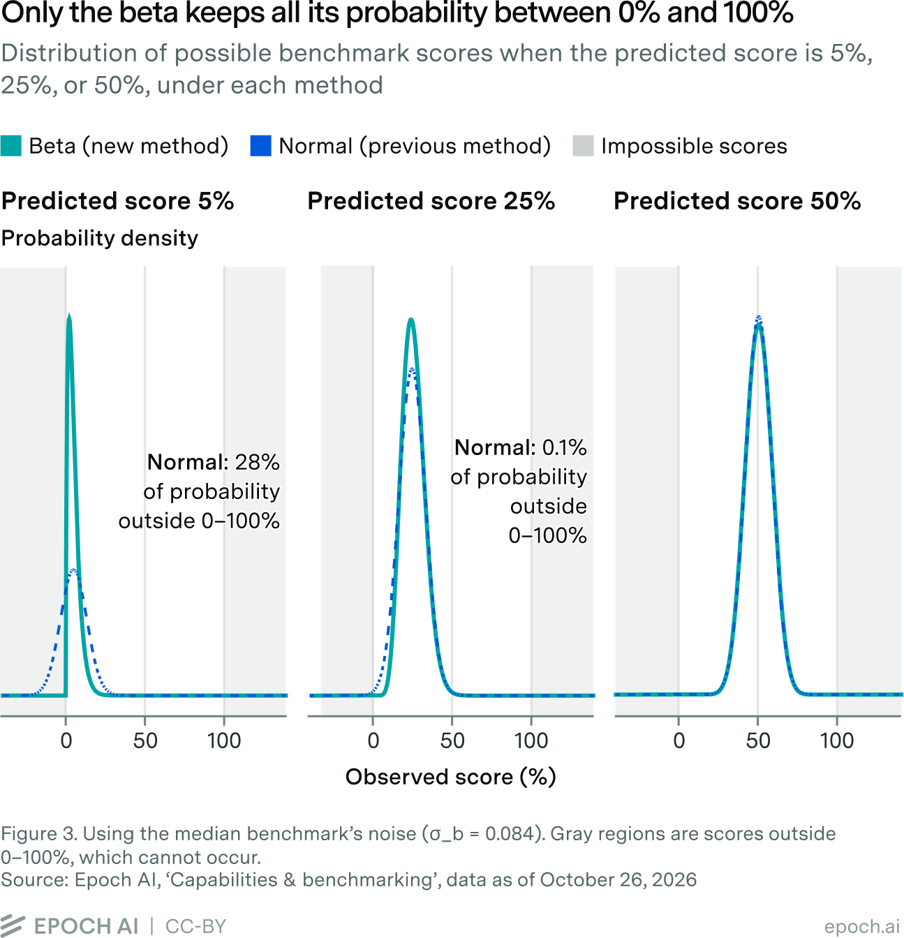
We set the predicted score function as the expected value (or mean) of our beta likelihood function, fit capability, difficulty, and slope parameters, and include benchmark-specific noise parameters, which we denote \(\sigma_b\) and discuss further in the next section. Then our likelihood is defined:
\[Y_{m,b} \mid \mu_{m,b}, \sigma_b \sim \mathrm{Beta}\left(\mu_{m,b}\,\frac{1 - 4\sigma_b^2}{4\sigma_b^2},\ (1 - \mu_{m,b})\,\frac{1 - 4\sigma_b^2}{4\sigma_b^2}\right)\]where \(\mu_{m,b} = \mathrm{predicted\_score}(m,b) = \sigma(\alpha_b[C_m - D_b])\).
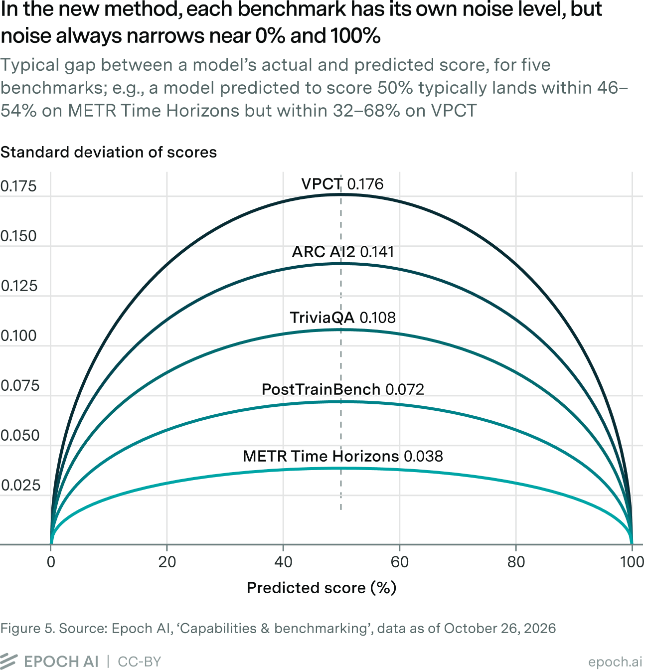
The mean of this likelihood is \(\mu_{m,b}\), and the standard deviation is \(2\sqrt{\mu_{m,b}(1 - \mu_{m,b})}\,\sigma_b\). The standard deviation (how much noise/error we expect in the benchmark results compared to the predictions) is maximized at \(\mu_{m,b} = \frac{1}{2}\) where it just equals \(\sigma_b\), and it shrinks to 0 as \(\mu_{m,b}\) goes to 0 or 1.
Finally, the beta distribution assigns no probability mass at exactly 0 or 1, so before fitting, we clip observed scores to [0.001, 0.999]. The ECI results are not sensitive to the exact range used here.
Each benchmark gets its own noise level
Benchmark-specific noise is another change we introduced to better match the model to patterns in the data. By ‘noise’ we mean how far a model’s observed scores tend to deviate from their predicted scores.
For example, a model predicted to score 50% typically lands within 46–54% on METR Time Horizons (taken as a % score on the task suite), while on VPCT it typically lands within 32–68%. In the previous frequentist fit, having the same penalty for every predicted-observed pair of scores effectively assumes that every benchmark is equally noisy. As our example shows, some benchmarks are noisier than others; by introducing the \(\sigma_b\) parameter, we can account for this in the model (Figures 4 and 5).
Note that even a benchmark with very little noise might still carry little information about a model that scores 99% on it, if, for example, almost any strong model would score near 99% too. A noisier benchmark on which the model scores 50% can tell us more. A score’s informativeness depends on the benchmark’s slope and how far the model’s capability is from the benchmark’s difficulty as well as its level of noise.

Fixing the scale with the full set of benchmarks
We fit the model on an internal ‘raw’ scale and then convert every sample to the final ‘ECI scale’ with a linear transformation that sets Claude 3.5 Sonnet to 130 and GPT-5 to 150. We do not fit on the ECI scale directly because the priors are more intuitive to set on the raw scale. Due to the way the predicted scores are calculated, they depend only on the difference between model capability and benchmark difficulty, multiplied by the benchmark’s slope. This means we could add a constant value to all the difficulty and capability parameters without changing any of the predicted scores, or similarly rescale everything by a constant factor and adjust the slopes. We need to remove situations like this, where different parameter values yield identical predictions, to sensibly fit our model.
In the previous frequentist model, we fixed the raw scale by setting WinoGrande’s benchmark slope at 1, alongside the regularization discussed above, which weakly set the mean of model capabilities and benchmark difficulty to zero5. In the new Bayesian model, we fix the geometric mean of benchmark slopes to 1: \(\prod_b \alpha_b = 1\) and center benchmark difficulties at zero: \(\sum_b D_b = 0\). This establishes the raw scale using the full set of benchmarks rather than relying on a single benchmark.
After fitting the model, we apply the same linear transformation as before to report results on the ECI scale, fixing Claude 3.5 Sonnet’s ECI at 130 and GPT-5’s ECI at 150. These anchors let us compare results over time, for example, when we receive more benchmark scores or a new model is released. Because these two anchors fix the scale, each model’s uncertainty interval describes its capability relative to Claude 3.5 Sonnet and GPT-5. The anchors themselves have no uncertainty.
Priors
In Bayesian modeling, we use priors, which are probability distributions that represent any existing knowledge we have for the plausible values. Setting priors describes what we expect before seeing the data. For the ECI, we do not have strong evidence of plausible values, and we do not want preconceived notions to have a substantial influence on results; instead, we want them to be data-driven. We therefore use flat priors on capability and difficulty, and loose hierarchical priors on the slopes and noise, which are probability distributions whose parameters (such as mean and variance) are themselves learned from the data.
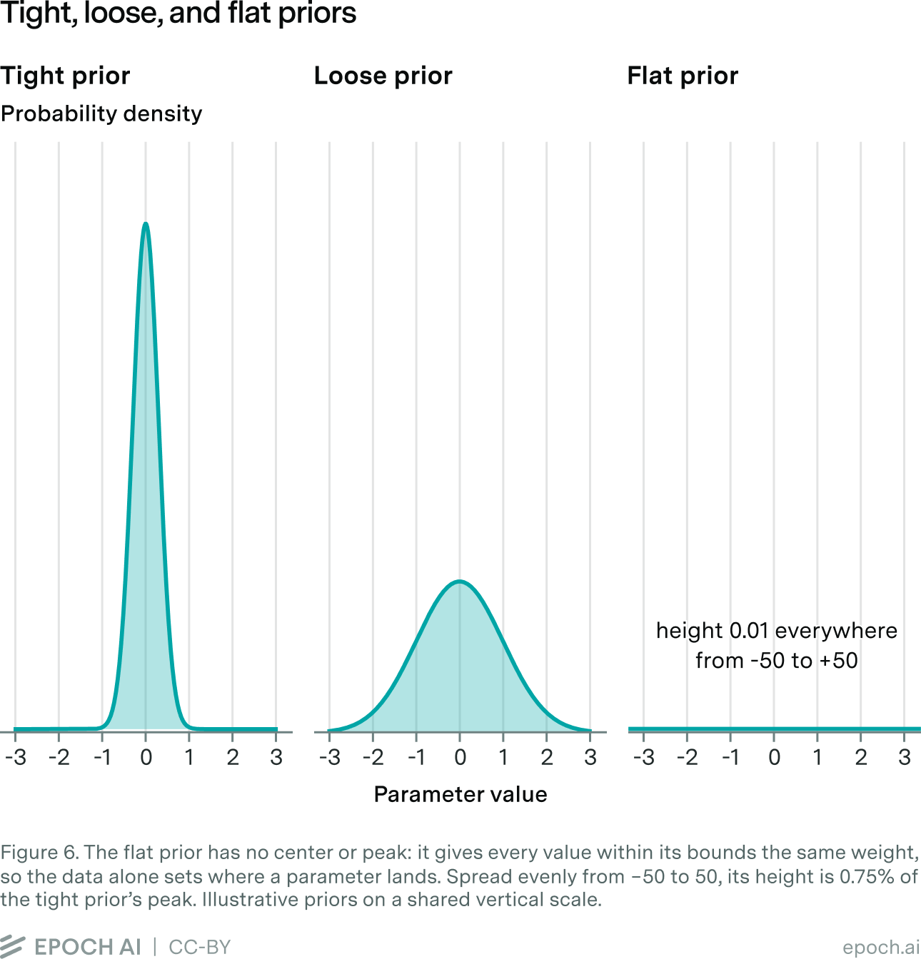
For capability \(C_m\) and difficulty \(D_b\), we want them to be roughly on the same scale. We set flat priors for these parameters, giving every value in a wide range the same probability, since we make no assumptions about how model capability or benchmark difficulty might be distributed. In particular, we don’t want the prior to constrain the rate of model progress that the model discovers. We then have
\[C_m, D_b \sim \mathrm{Uniform}(-50, 50).\]We bound the priors so the posterior stays well defined, but set the bounds far wider than the data can reach: when converted from the raw scale to the ECI scale with the current fit, they span ECI values of −390 to +670, while the models in our data sit between about 45 and 169.
For the slope parameter, we do have some prior knowledge: we expect benchmarks to cluster around a typical rate of change, and a benchmark whose scores change 100 times faster or slower than average would be surprising. A natural prior for a slope parameter such as \(\alpha_b\) is the log-normal: it is strictly positive, it treats “twice as fast” and “half as fast” symmetrically, and it can span several orders of magnitude. Rather than fix how spread out the slopes are, we learn that from the data with a hyperprior. We set \(\tau_\alpha\) to be the scale parameter, and set 0 as the location parameter, so that
\[\alpha_b \sim \mathrm{LogNormal}(0, \tau_\alpha) \quad \text{marginally, with} \quad \tau_\alpha \sim \mathrm{LogNormal}(\log(0.5), 0.5).\]Finally, for the per-benchmark noise parameter, we use a log-normal with hyperpriors for the location and spread:
\[\sigma_b \sim \mathrm{LogNormal}(\log \sigma_{\mathrm{median}}, \tau_\sigma) \ \text{truncated between } (0, 0.5),\]with
\[\sigma_{\mathrm{median}} \sim \mathrm{LogNormal}(\log(0.1), 0.5) \quad \text{and} \quad \tau_\sigma \sim \mathrm{LogNormal}(\log(0.5), 0.5).\]Because these priors have their own learned parameters, the model is hierarchical. We chose fixed hyperparameters via grid search; the results are not sensitive to them.
Frontier ECIs barely move, and models can now be compared
This section covers the impacts of switching from the old frequentist model to the new Bayesian model. We assess how individual ECI values changed, how the frontier trend changed, how well the new model fits the data, and what the joint posterior lets us say when comparing models.
Frontier ECIs are similar while weak models move down
The Bayesian model affects two groups of models very differently, with GPT-4 as the dividing line. GPT-4 is the earliest model in our frontier trend and the weakest frontier model in our dataset (ECI 126 under the previous frequentist method, 122 with the Bayesian fit). Models below this were behind the frontier when they were released.
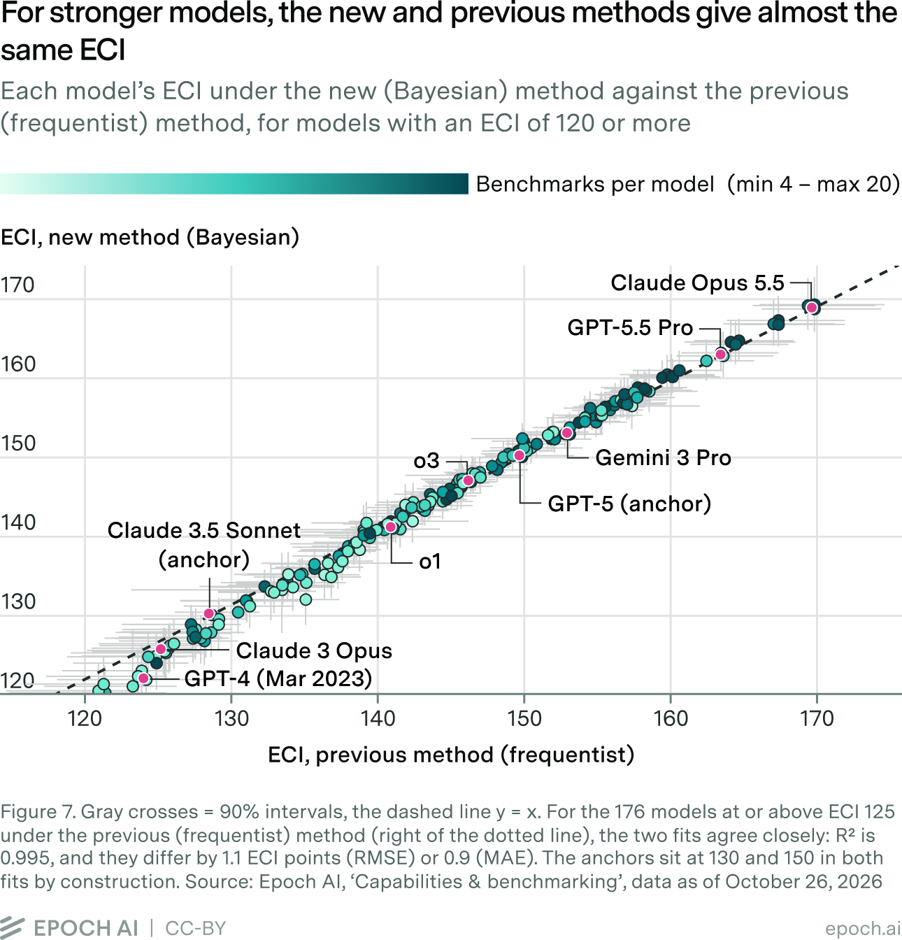
Models at ECI 125 and above
For the 176 models at or above ECI 125, the two fits agree closely. Figure 7 plots each model’s new ECI against its previous ECI. The points sit on the diagonal (R² 0.995), and the two fits differ by 1.1 ECI points by root mean squared error (RMSE) and 0.9 by mean absolute difference. Every model’s new ECI lies inside its previous 90% confidence interval, typically a quarter of the way from its center to its edge, and the new intervals are 13% narrower on average. Models above ECI 150 tend to move up slightly: 87% of them do, by 0.7 points on average and at most 2.3.
Models below ECI 125
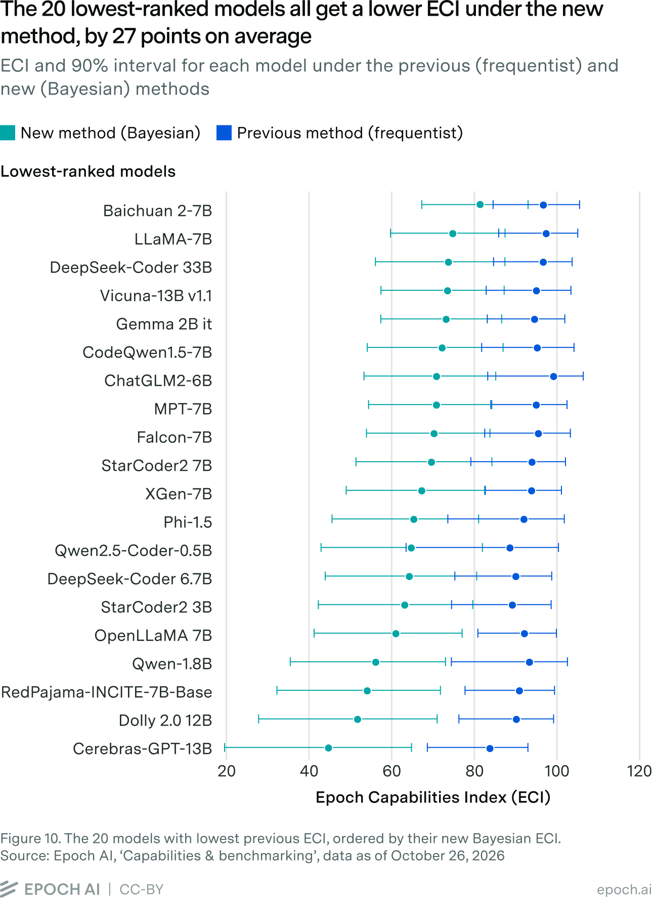
The 76 models below ECI 125 all move down, by 13.7 points on average, and by 27 points for the 21 models previously below 100 (Figure 8; Figure 10 shows the 20 weakest models). The weaker a model, the further it moves: the change stretches the bottom of the scale rather than shifting these models by a fixed amount.
Part of this change comes from dropping the previous fit’s regularization: the penalty on large parameter values and their bounds. That penalty pulled every capability toward zero on the raw scale, which mattered little for models with many scores but held up very weak models measured on a few, mostly saturated, benchmarks. Refitting the previous frequentist model without the penalty and bounds moves models below ECI 100 down by 10.5 points (from 27 under the Bayesian fit) and models between 100 and 125 down by 3.6 points (from 8.8). The rest of the change comes from the new model itself. We could have kept a penalty to prevent this change, but we did not think it was a justified feature of the original frequentist model: it pulls a model toward the average simply because it has few scores. It also doesn’t affect anything the ECI is typically used for, since these models sit well below the frontier.
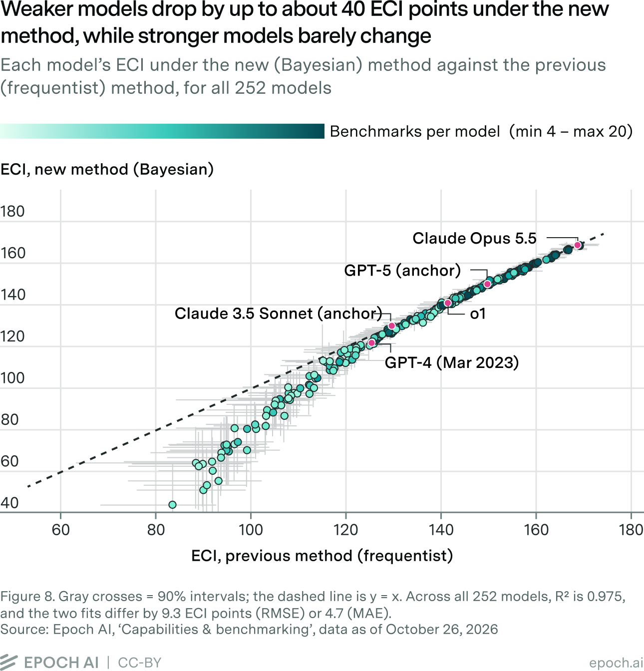
The table below compares the two groups.
| Previous ECI | Models | Mean change | Mean absolute change | Largest change | Change in average 90% interval width |
|---|---|---|---|---|---|
| 125 and above | 176 | -0.1 | 0.9 | -4.1 | -13% |
| Below 125 | 76 | -13.7 | 13.7 | -39.2 | +33% |
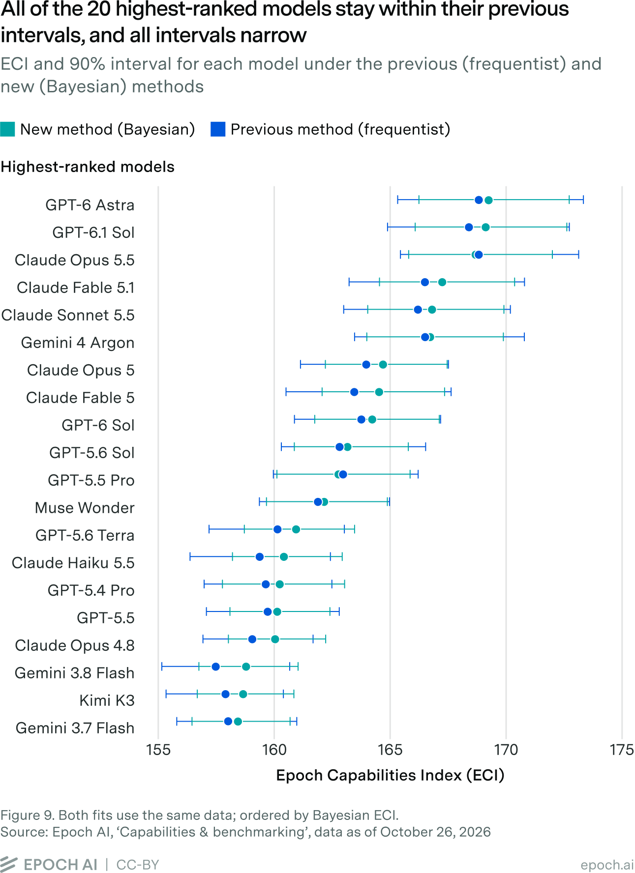
Figures 9 and 10 show each model’s ECI and 90% interval under both fits, for the 20 highest-ranked models and the 20 weakest. All 20 top models lie within their previous intervals; 18 move up slightly, by 0.7 points on average, and all 20 get narrower intervals. The 20 weakest models (by previous ECI) all move down, by 27 points on average, and all 20 get wider intervals.
Frontier trends get slightly steeper
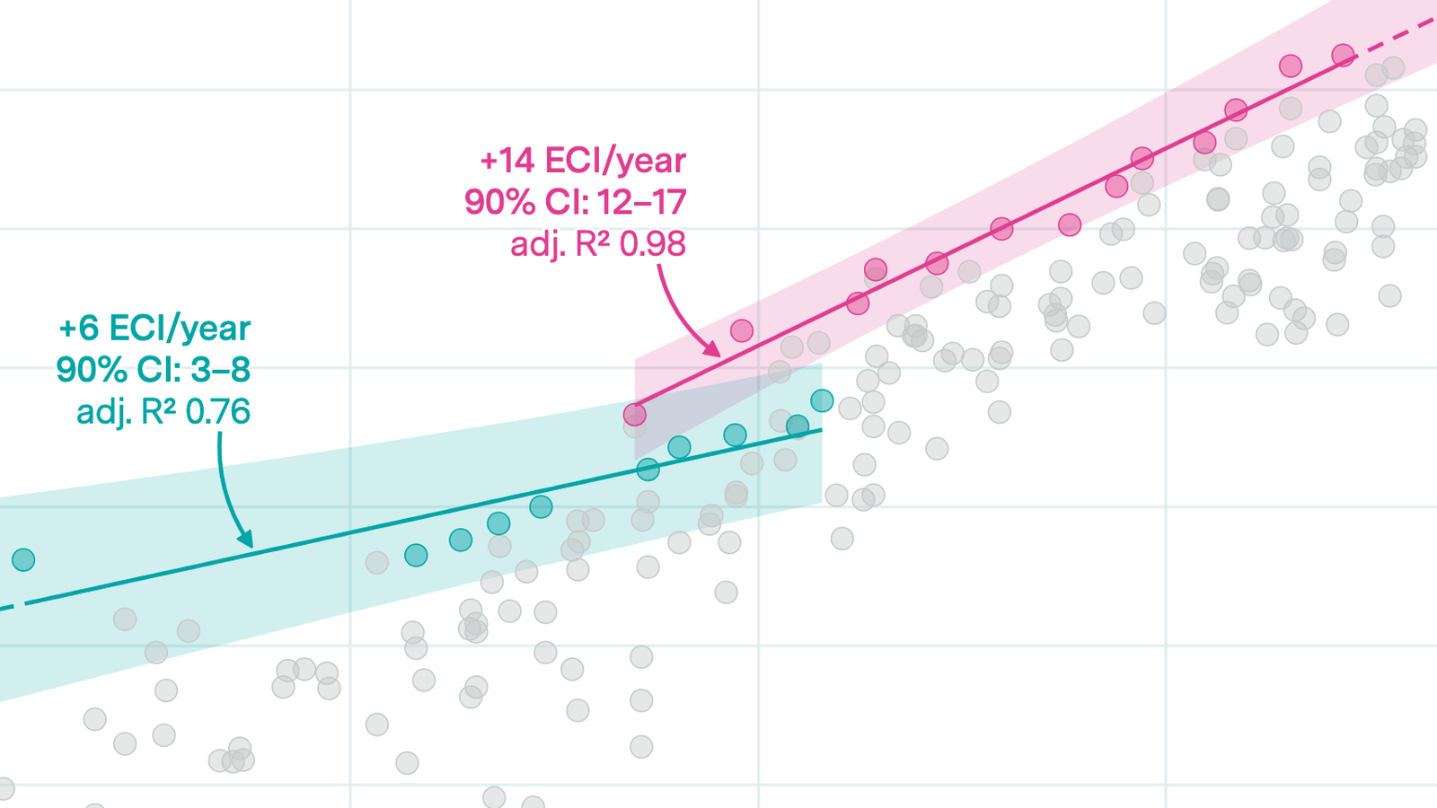
We refit the frontier trend with the same criteria as our prior work analyzing trends in the ECI6, using the Bayesian model. We fit separate trends for reasoning and non-reasoning models, ending the non-reasoning trend at GPT-4.5.
Figure 11 shows each era’s trend under the frequentist and Bayesian fits, and the table below gives both eras’ trends.

| Era | Frequentist ECI/year (90% intervals) | Bayesian ECI/year (90% intervals) |
|---|---|---|
| Pre-reasoning (GPT-4 to GPT-4.5) | 6.2 (2.8–7.8) | 8.0 (5.4–9.7) |
| Reasoning (from o1-mini) | 15.7 (13.8–19.2) | 16.6 (14.6–18.7) |
Both trends get about one to two ECI points per year steeper, which is small compared to their uncertainty. This is likely due mainly to a change of scale: the Bayesian fit places the two anchor models, Claude 3.5 Sonnet and GPT-5, closer together in capability compared to the frequentist fit. Because both fits fix the gap between these two anchors at 20 ECI points, the Bayesian scale stretches relative to the frequentist one. For example, GPT-4 and Claude Opus 5.5 have a 46.9-point ECI gap in the Bayesian fit, compared with 43.0 in the frequentist fit.
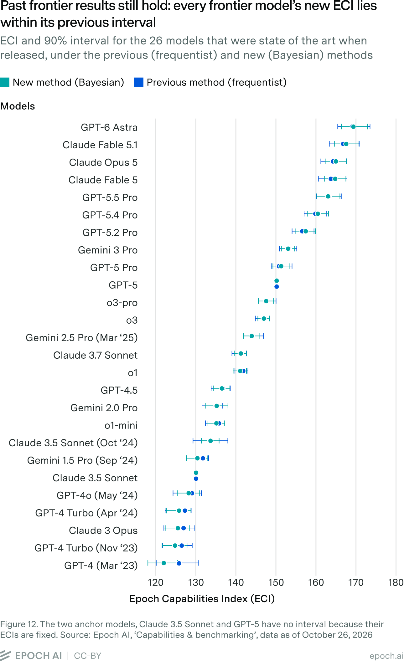
Within each era, earlier frontier models move down slightly and later ones up: GPT-4 drops 4.0 points while GPT-4.5 drops 0.2, and the first half of the reasoning-era frontier moves by −0.1 on average against +0.5 for the second half. The two fits also pick slightly different frontier models because each draws from its own estimates. Each frontier model’s new ECI lies within its previous 90% interval (Figure 12).
Similar accuracy, better calibrated out of sample
The main reason for moving to a Bayesian model was to get better-justified uncertainty estimates. In this section, we assess both the accuracy of the predicted scores and the calibration of their uncertainty, comparing the previous frequentist approach with the new Bayesian one.
Accuracy measures how far predicted scores are from the observed scores, using RMSE and mean absolute error (MAE). Calibration measures whether the uncertainty is right. For each observed score, the fit gives a range that should contain it 90% of the time. If the fit is well calibrated, about 90% of observed scores fall inside their range; much more means the ranges are too wide, and much less means they are too narrow. The frequentist fit gives only a single predicted score, with no range, so to compare we treat each prediction as a normal distribution with the same spread (SD 0.076) for every score, as described in the section on the beta likelihood. We check calibration for all scores, and separately for scores near 0 and 1, where a single noise level for every score fits worst. In-sample results check each score against a fit that included it; leave-one-out results check it against a fit that didn’t, which tests how well each fit predicts scores it has not seen.
| Frequentist in-sample | Frequentist leave-one-out | Bayesian in-sample | Bayesian leave-one-out | |
|---|---|---|---|---|
| RMSE (lower is better) | 0.076 | 0.094 | 0.079 | 0.092 |
| MAE (lower is better) | 0.057 | 0.068 | 0.058 | 0.067 |
| Beta-scaled RMSE7 | 0.097 | 0.117 | 0.093 | 0.108 |
| 90% coverage, all scores (90% target) | 90.5% | 84.2% | 94.4% | 89.6% |
| 90% coverage, scores ≤ 5% (90% target) | 95.0% | 92.5% | 87.5% | 80.5% |
| 90% coverage, scores ≥ 95% (90% target) | 98.2% | 98.2% | 94.7% | 93.0% |
In-sample, the frequentist fit has a slightly lower error; however, out of sample, the Bayesian model is slightly better. The Bayesian intervals contain 89.6% of out-of-sample scores, against 84.2% for the frequentist fit. Near 0 and 1, the frequentist intervals contain almost every score because they extend below 0 and above 1 into impossible values, as discussed in the section on the beta likelihood. The Bayesian intervals stay within the possible range and contain 80.5% of scores near 0 out of sample.
How likely one model is to be more capable than another
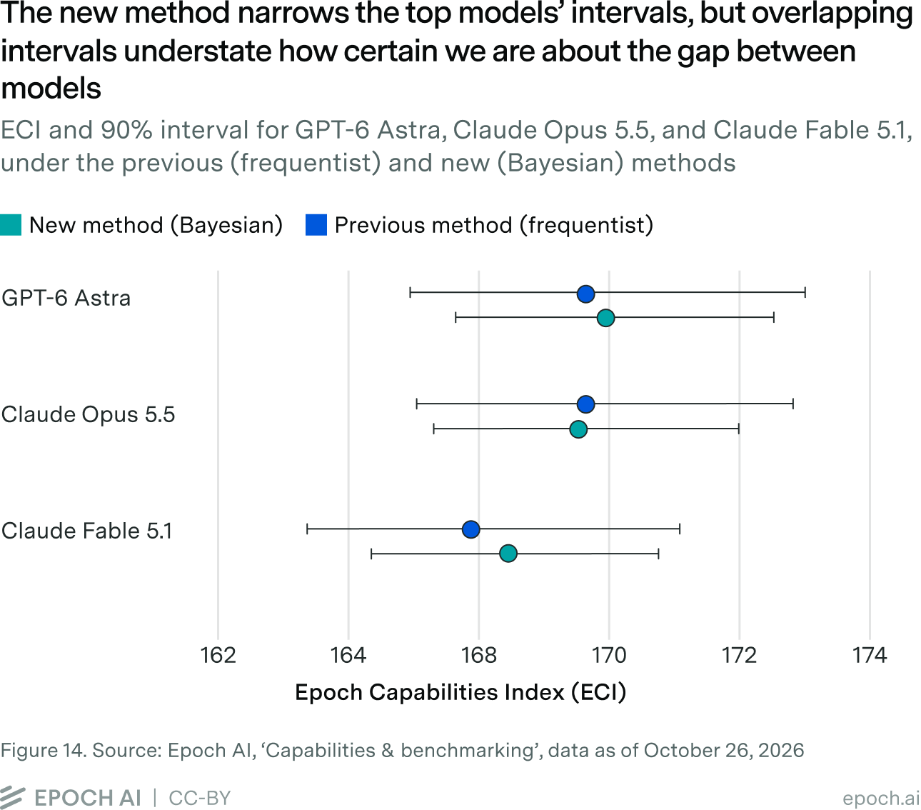
The Bayesian fit gives a probability distribution for each model’s ECI. Figure 13 shows these distributions for the 20 highest-ranked models. Wider distributions mean more uncertainty. These distributions are still fairly wide and often overlap: GPT-6 Astra’s 90% interval runs from 166.2 to 172.7, and Claude Opus 5.5’s from 165.8 to 172.0 (Figure 14).
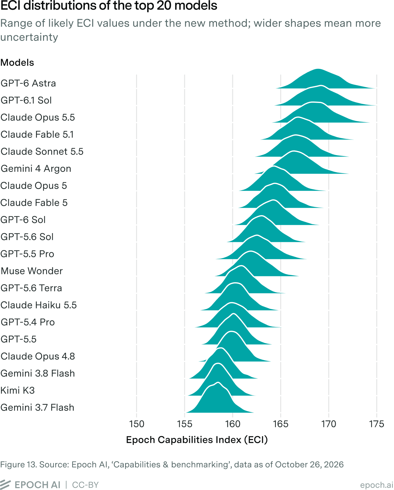
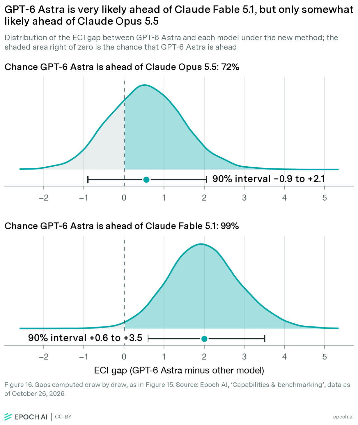
We are often much more certain about the gap between two nearby models than their separate intervals suggest. Much of each model’s uncertainty is shared across models, as it comes from uncertainty in the gap between the two anchor models, Claude 3.5 Sonnet and GPT-5. Because that gap is fixed to be exactly 20 ECI points, a draw in which the anchors sit closer together on the raw scale stretches the whole scale, and models near each other move together, so the gap between them is less uncertain than either model’s ECI. The 90% interval for the gap between GPT-6 Astra and Claude Opus 5.5 runs from −0.9 to +2.1, half the width of either model’s own interval.
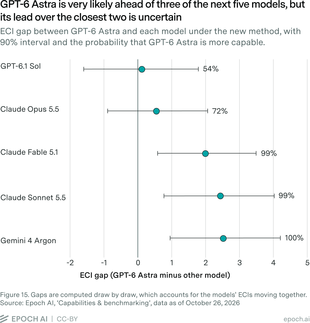
Because we estimate each model’s capability together, we can now compare models directly. Figure 15 shows the five models closest behind GPT-6 Astra, which has a 72% probability of being more capable than Claude Opus 5.5, but a 99% probability of being more capable than Claude Fable 5.1. Figure 16 shows the full probability distribution of these two gaps. We hope to present more results like this alongside the ECI in the future.
Conclusion: better uncertainty, similar frontier ECIs
We have updated the ECI modeling to use a Bayesian model. The index itself works the same way: each model has a single capability score, each benchmark has a difficulty and a slope, and the scale is anchored to Claude 3.5 Sonnet at 130 and GPT-5 at 150. What has changed is how we fit it and how we calculate uncertainty.
Three major takeaways from the update are:
- Uncertainty estimates are better justified. They come from a single model that uses all the data at once, rather than resampling the handful of scores each model has. They are narrower than before for models near and above the anchors, and wider for models with few benchmark scores.
- Models can be compared directly. We estimate all capabilities together, so we can say how likely one model is to be more capable than another, and by how much.
- ECI values and trends hold. For models at ECI 125 and above, which include every frontier model, ECIs move by about one point on average and always stay inside their previous intervals. The frontier trend is one to two ECI points per year steeper, which is a small shift compared to previous uncertainty estimates. The biggest changes are among older, very weak models that were never close to the frontier, which now sit lower.
The Bayesian model is a strong base for further extensions to the ECI and new uses of its results, which we look forward to sharing. The new ECI, data, and code are available on our website.
Appendices
Appendix A: Alternative models
The model in the main text came out of several rounds of exploration of priors and likelihoods. This appendix covers the main alternatives we tried and why we didn’t adopt them. We first describe the change from normal to uniform priors on capability and difficulty (A1.1). We then compare alternative likelihoods: how fast noise should shrink near 0 and 1 (A1.2), how the likelihoods compare overall (A1.3), and whether to put probability exactly on 0 and 1 (A1.4). We ran these comparisons under normal priors; under uniform ones, three of the five alternatives failed to converge and the other two mixed very slowly, while the beta likelihood was unaffected. We evaluated each likelihood at its best-fitting settings.
These experiments use data from October 14, 2026; therefore, some metrics and numbers differ slightly from the main model and Appendix B. Coverage is also checked differently. The main text and Appendix B check coverage against the scores the model was fitted to, where exact zeros are clipped just above 0. Here we check it against the scores as reported. The beta’s intervals can never include exactly 0, so each reported zero counts as a miss, and the beta’s coverage is about 3 points lower here.
A1.1 Normal to uniform priors
We first developed the beta model with hierarchical normal priors on capability and difficulty, whose spread was itself learned from the data. These priors pull each model toward the average unless strong evidence suggests otherwise. The pull grows in proportion to how far a model sits from the average, and weakens the more its scores pin it down. It therefore moves the weakest models most, since they sit far below the average and often have only a few scores, too.
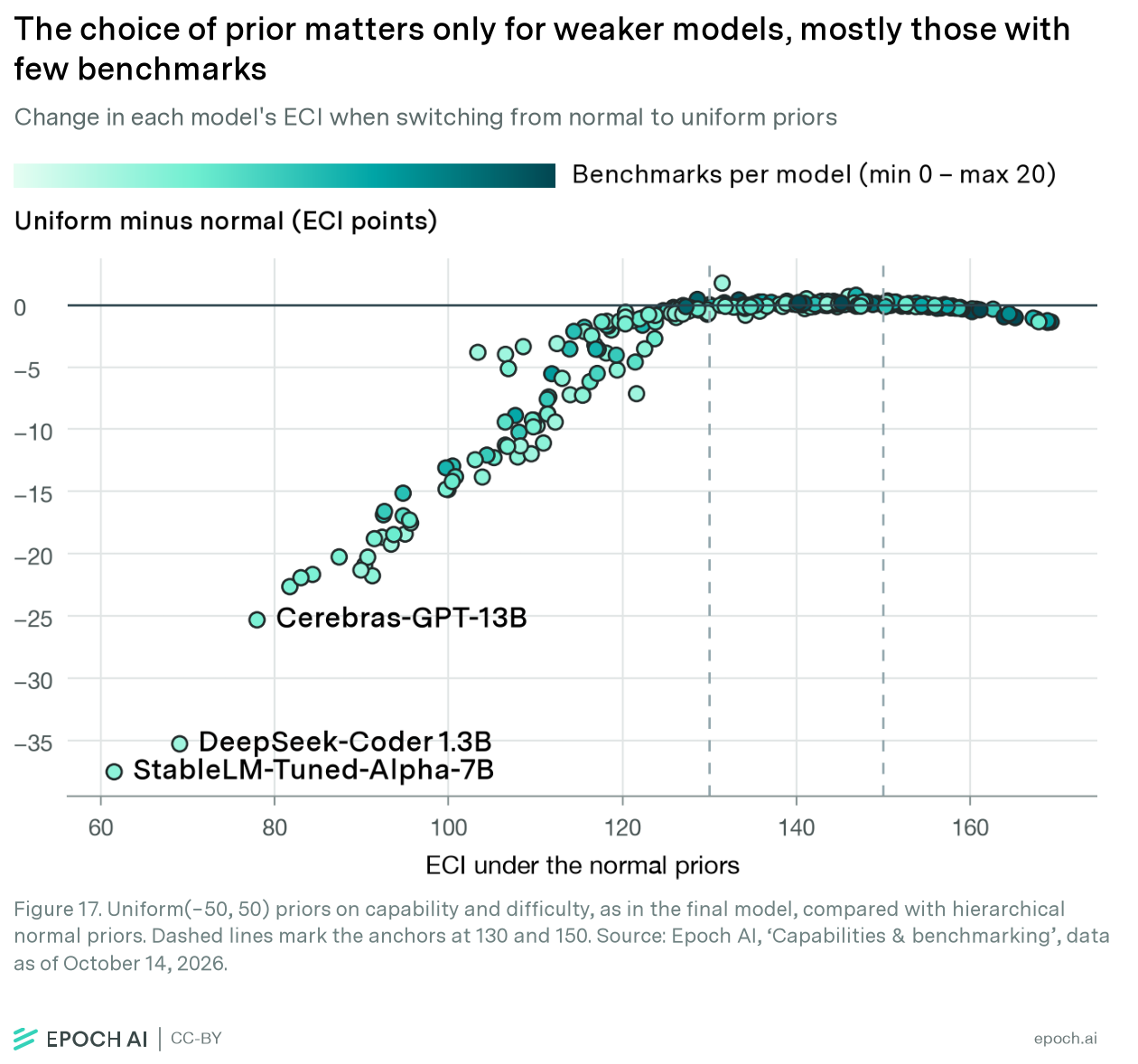
We switched to the Uniform(−50, 50) priors described in the main text, which assume nothing about how capabilities or difficulties are distributed. The switch leaves the frontier almost untouched: models above ECI 130 move by less than 0.3 points on average. The changes are concentrated among weak models scored on a few older benchmarks. Under uniform priors, models between ECI 100 and 130 sit about 4 points lower, and models below 100 about 20 points lower (Figure 17). The data alone cannot distinguish the two priors, as both fit the observed scores almost equally well. We chose the uniform because it lets the scores, not the prior, set how weak these models are. This also matters for future frontier models: as they move further above the average, a normal prior could pull them down.
A1.2 How fast should noise shrink near 0 and 1?
The beta’s noise shrinks toward 0 and 1 at a rate fixed by its shape. To test whether that rate is right, we need a likelihood where the rate is a free parameter. We use a normal distribution truncated to [0, 1], with a power-variance term:
\[\text{standard deviation} = \sigma_b \left(4\mu(1 - \mu)\right)^p\]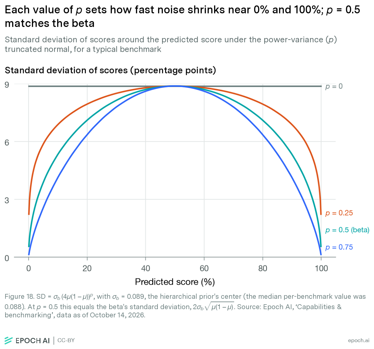
At a predicted score of \(\mu = 0.5\), the term in brackets equals 1, so \(\sigma_b\) is the benchmark’s noise in the middle of the range. The exponent p sets how fast the noise shrinks toward the boundaries (Figure 18). With p = 0, the noise is the same everywhere, as in least squares. With p = 0.5, the formula is exactly the beta’s standard deviation, \(2\sigma_b\sqrt{\mu(1 - \mu)}\).
| p | ELPD vs p = 0.5 (higher is better) | RMSE (in-sample) | RMSE (PSIS-LOO) | 90% coverage, all scores (in-sample) | 90% coverage, near 0 (in-sample) |
|---|---|---|---|---|---|
| 0.25 | Did not converge | ||||
| 0.50 | 0 | 0.0798 | 0.0924 | 91.6% | 69% |
| 0.55 | -3 ± 3 | 0.0800 | 0.0927 | 91.7% | 69% |
| 0.75 | -22 ± 14 | 0.0819 | 0.0937 | 91.5% | 66% |
| Beta for reference | n/a | 0.0788 | 0.0917 | 91.2% | 88% |
Table A2. Truncated normal at several values of p, under the final model’s uniform priors and sampler settings. ELPD differences are paired against p = 0.5, ± one standard error.
Predictive fit (ELPD, higher is better) peaks at around p = 0.5. That is the beta’s own rate, so the beta already gets the shape of the noise about right. Noise that shrinks faster (p = 0.75) fits clearly worse. Noise that shrinks more slowly made the model hard to fit at all: at p = 0.25 the sampler failed to converge. An earlier sweep under normal priors, on an older data snapshot, showed fit improving steadily from p = 0.05 up to 0.5. Accuracy and overall coverage barely change with p. No value of p fixes the scores near 0: about a third of them fall outside the 90% intervals at every p, against an eighth for the beta. Changing how fast noise shrinks doesn’t help with scores that sit at the boundary, which is what A1.4 addresses.
A1.3 Comparing the likelihoods
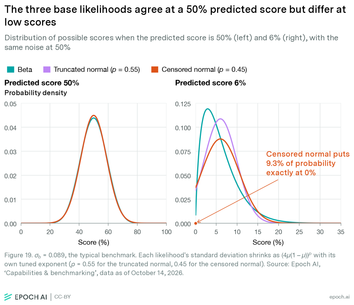
We compared the beta against five alternatives (Figure 19 shows the three base likelihoods):
- Truncated normal, described in A1.2;
- Censored normal, described in A1.4;
- Three different combinations of the beta, the truncated normal and the censored normal. For these mixture distributions, where each score comes from one of several components, the mixing weights are also learned from the data.
We found these often had convergence issues with uniform priors, so we compare them here under normal priors. These still produced some divergent draws (14 for the truncated normal, 3 for the censored normal), but were stable enough for comparison.
| Likelihood | RMSE | CRPS | 90% coverage, all scores |
|---|---|---|---|
| Beta with normal priors | 0.0798 | 0.0411 | 91.7% |
| Truncated normal | 0.0794 | 0.0407 | 90.5% |
| Beta + truncated normal | 0.0788 | 0.0402 | 91.3% |
| Censored normal | 0.0781 | 0.0402 | 94.2% |
| Beta + censored normal | 0.0786 | 0.0400 | 94.8% |
| Beta + truncated normal + censored normal | 0.0782 | 0.0399 | 95.1% |
| Beta with uniform priors | 0.0788 | 0.0406 | 91.2% |
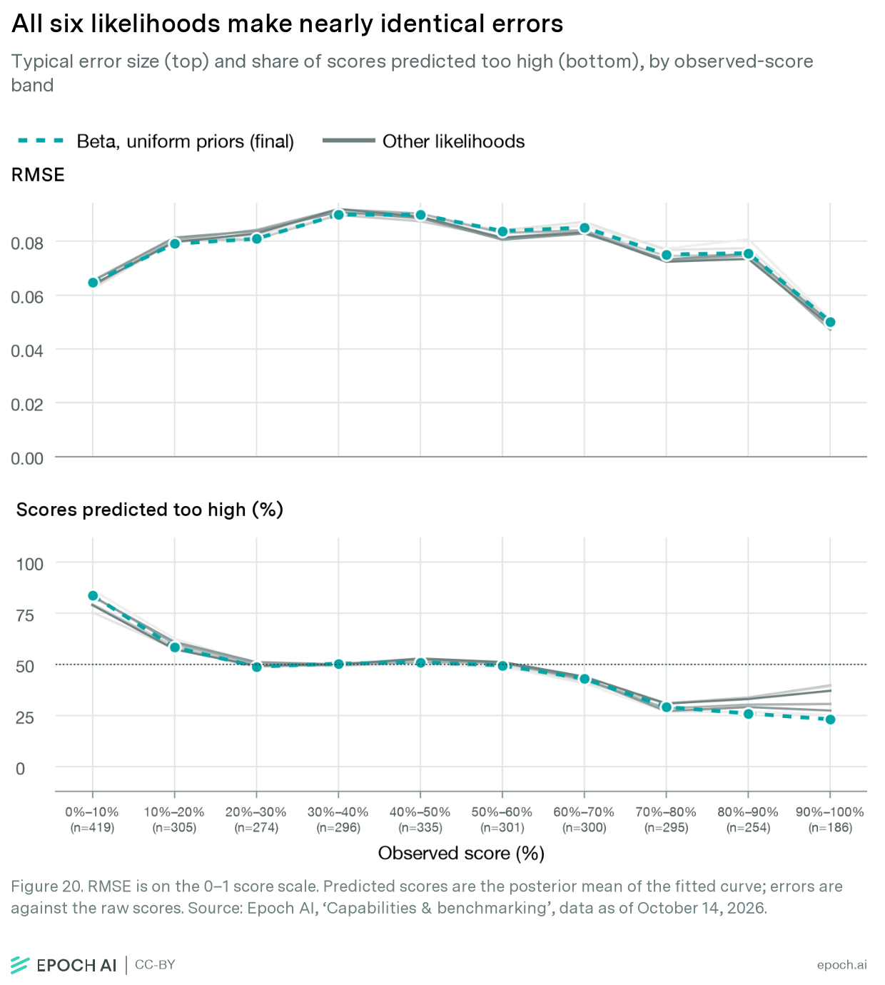
All likelihoods predict scores similarly: RMSE varies by 0.17 percentage points, and CRPS (an accuracy measure that scores the whole predicted distribution) by 0.12. For all, about 70% of the error comes from scores between 0.2 and 0.8 (Figure 20).
A1.4 Probability exactly at 0 and 1
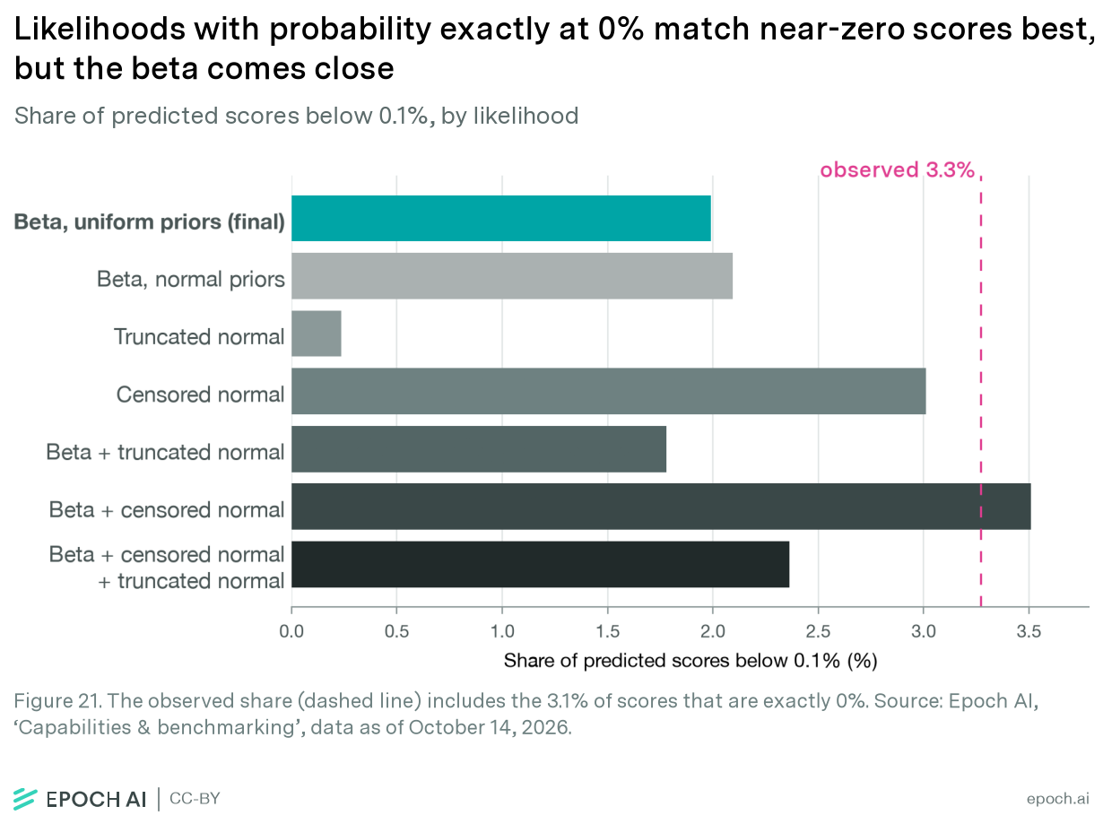
A continuous likelihood such as the beta gives zero probability to any single value, so it can never predict a score of exactly 0, yet 3.1%8 of observed scores are exactly 0. A censored normal takes the probability that would fall below 0 and places it exactly at 0, and likewise at 1. These point masses (atoms) let the model predict exact zeros directly. Figure 21 compares the share of scores each likelihood predicts below 0.1% with the observed 3.3%, almost all of them exact zeros. Likelihoods with atoms predict 2.4–3.5%, the beta 2.0–2.1%, and the truncated normal almost none (0.2%).
| Likelihood | Predicted share of exact zeros | 90% coverage, near 0 | 99% coverage, all scores |
|---|---|---|---|
| Without atoms (beta, truncated normal, beta + truncated normal) | 0% | 52–58% | 96% |
| With atoms (censored normal, beta + censored normal, all three) | 2.0–3.5% | 91–95% | 99.1–99.7% |
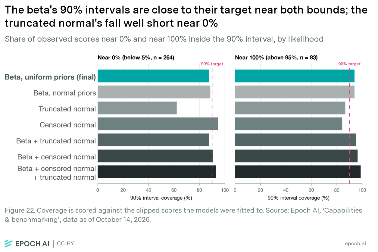
Coverage near 0 is scored against the raw scores, so a likelihood without an atom can never cover a score of exactly 0. Scored against the clipped scores the models were fitted to, the beta covers 89% of scores near 0 under normal priors and 88% under uniform priors (Figure 22).
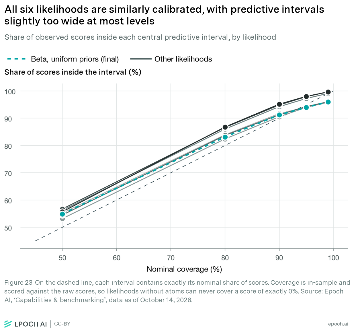
Atoms predict roughly the right share of exact zeros and give better intervals near 0, but only for the weakest models. Elsewhere they make the intervals too wide (Figure 23).
Why we kept the beta likelihood
No alternative likelihood improves on the beta enough to justify its extra complexity. The beta already shrinks noise at about the rate the data prefers, and the alternatives predict scores and rank models almost identically. Atoms do give better intervals at exactly 0, but only for the weakest models, and they miscalibrate elsewhere. Finally, with the uniform priors, which are better justified, the beta is the only likelihood that samples reliably.
Appendix B: Implementation, data and evaluation
This appendix gives the details needed to reproduce and assess the final model. We describe how we implement and fit it, where the data comes from and how it’s pre-processed, and how it is evaluated. The evaluation covers whether the sampler explored the posterior properly, how accurately the model predicts the observed scores, and whether its uncertainty matches the data. Where applicable, we compare against the previous frequentist fit on the same data.
Implementation
We implement the model in PyMC and fit it using the NUTS sampler with 4 chains, a target accept rate of 0.95, and a max tree depth of 10. The model can be fit with a single run using PyMC’s default diagonal mass matrix, but that needs about 12,000 draws per chain to pass the convergence checks below. This is because the capability, difficulty, and slope parameters are strongly correlated, and a diagonal mass matrix ignores these correlations.
To speed up the fitting, we instead fit the model in two runs:
- Pilot run: 1,000 tuning steps and 1,000 draws per chain with the default diagonal mass matrix. We use its draws only to estimate the correlations between parameters and to start each main-run chain from a different point.
- Main run: 500 tuning steps, then 1,000 draws per chain, using the correlations from the pilot run for a dense mass matrix.
This speeds up the sampling but does not change the results. We require no divergences, a bulk ESS of at least 400 for every parameter, and R̂ of at most 1.01. If the main run misses these checks, it reruns with more draws, up to 16,000 per chain. As a last resort, we fit the model with the default diagonal mass matrix alone, with up to 32,000 draws per chain. The final fit passed the checks on the first main run with the dense mass matrix at 1,000 draws per chain.
Sampling takes about a minute (56 seconds for the pilot run, 13 for the main run) on an M5 MacBook Pro. With these settings, the fit has no divergences, a bulk ESS of 1,230 and a tail ESS of 1,289 at the lowest, and E-BFMI between 0.83 and 0.91 per chain. The sampler never needed a tree deeper than 5. The highest R̂ is 1.005.
Data processing
We get live data from our benchmark hub. Benchmark scores are partly sourced from independent third parties, some are run by Epoch AI, and for a few historical benchmarks we use scores reported by model developers. The data is pre-processed and updated regularly. For more information, see our data page. This write-up is based on data accessed on October 26, 2026, comprising 2,810 scores, 252 models, and 59 benchmarks.
Before fitting, we process the scores in four steps:
- Normalize each score so that the benchmark’s random-guessing baseline maps to 0 and its maximum achievable score maps to 1. Scores below the baseline are set to 0, and scores above the maximum to 1.
- Where a model has several versions, we keep its best score on each benchmark.
- We keep only models with scores on at least 4 benchmarks, of which at least 4 are between 0.1 and 0.9. Models that qualify keep all their scores.
- We clip scores to [0.001, 0.999].
Evaluation
There are three main categories of metrics that we use to assess goodness of fit: sampling metrics, predictive accuracy, and calibration.
Sampling
We evaluate sampling quality by how well the chains explore the probability space. While these metrics do not tell us if the model is optimized for accuracy, if sampling metrics fail, then we can’t trust metrics downstream; we need to fix the sampling first, otherwise we are evaluating incomplete distributions.
| Check | Good value | Our result |
|---|---|---|
| R-hat (highest across parameters) | 1.01 or below | 1.005 |
| Bulk ESS (lowest across parameters) | 400 or above | 1,230 |
| Tail ESS (lowest across parameters) | 400 or above | 1,289 |
| Divergences | 0 (hard cut-off) | 0 out of 4,000 draws |
| E-BFMI (each chain) | Above 0.3 | 0.83 to 0.91 |
| Moves that hit the tree depth limit | 0% | 0% |
Quality of fit
Prediction accuracy checks how close the model’s predicted scores are to the observed scores in the data, and then outputs the average over all predicted-observed pairs as a metric reflecting quality of prediction9. Performance scores range from 0 to 1, so an error of 0.05 means the prediction is 5 percentage points from the actual score.
| Metric | What it measures | Frequentist (in-sample) | Frequentist (exact LOO) | Bayesian (in-sample) | Bayesian (PSIS-LOO) |
|---|---|---|---|---|---|
| Median absolute error | How far off a typical prediction is | 0.043 | 0.050 | 0.043 | 0.050 |
| MAE (mean absolute error) | How far off predictions are on average | 0.057 | 0.068 | 0.058 | 0.067 |
| RMSE (root mean squared error) | Like MAE, but large misses count for more | 0.076 | 0.094 | 0.079 | 0.092 |
| Mean bias | Whether predictions are too high or too low on average (0 means neither) | +0.001 | +0.000 | -0.001 | -0.001 |
| CRPS10 | How close the full range of predicted scores is to the real score | n/a | n/a | 0.041 | 0.048 |
| ELPD11 per score | Log density assigned to each real score, when that score is left out of the fit (higher is better, but only meaningful when compared to other models) | n/a | n/a | n/a | 1.21 |
To check whether the model’s uncertainty matches the data, we compare each observed benchmark score with the range of scores the model predicts for it. If the model is well calibrated, 90% of observed scores should fall within their 90% predicted interval, and the same should hold at other levels. The in-sample column checks each score against a fit that included it. The leave-one-out column checks each score against a fit that left it out, testing how well the model predicts unseen scores. Refitting the model once for each of the 2,810 scores would be computationally intensive, so we approximate the leave-one-out fits with PSIS-LOO, which reuses the draws from the single full fit. On an earlier version of the model, exact leave-one-out refits gave coverage within about a percentage point of the PSIS approximation.
| Range | Ideal coverage | In-sample Bayesian fit | Leave-one-out Bayesian fit |
|---|---|---|---|
| 50% | 50% | 56.3% | 50.8% |
| 80% | 80% | 86.0% | 79.9% |
| 90% | 90% | 94.4% | 89.6% |
| 95% | 95% | 97.4% | 94.4% |
| 99% | 99% | 99.4% | 98.3% |
We also check the PIT (probability integral transform) and PPP12 (posterior predictive p-values).
| Statistic | Ideal score | Our results |
|---|---|---|
| PIT KS statistic | Lower (0) is better | 0.0418 |
| Mean PIT | Closer to 0.5 is better | 0.5087 |
| PPP, variance | Closer to 0.5 is better | 0.565 |
| PPP, IQR | Closer to 0.5 is better | 0.078 |
-
See Appendix B for more detail.

-
No-U-Turn Sampler (NUTS) on PyMC. Further sampler settings and diagnostics are in Appendix B.
-
Confidence intervals used in frequentist modeling are replaced with credible intervals in Bayesian modeling, and can be computed as the highest density interval (HDI) or as equal-tailed intervals (ETI). We use the latter.
-
We also tested likelihoods that place probability mass exactly at 0 and 1 (called atoms) to predict exact zeros. See A1.4 in Appendix A for details.
-
Scale parameters were also restricted to [0.1, 10] and capability and difficulty to [−10, 10], but this didn’t impact the model fit.
-
We follow the published classification, and additionally treat DeepSeek-R1’s distilled models (released alongside it in January 2025) as reasoning models.
-
Squared errors divided by 4y(1−y), where y is each fit’s own predicted score, so misses near 0 and 1 count for more, as in the beta likelihood.
-
From October 14, 2026 data, this number can vary as new data is added.
-
In-sample metrics may look better than leave-one-out ones, so we give both. Frequentist leave-one-out values come from refitting the model once per score; Bayesian ones use PSIS-LOO, which approximates those refits by reweighting the draws from the single full fit (see the calibration check below). Least squares has no predictive distribution, so it has no CRPS or ELPD.
-
The average distance between the predicted distribution and the observed score, in score units; it reduces to the absolute error when the prediction is a single number.
-
How much probability the model gives each score when that score is left out of the fit. It is approximated with Pareto-smoothed importance sampling rather than 2,810 refits. Only differences between models fitted to the same data are comparable.
-
See section 6.3.
About the authors


Related work