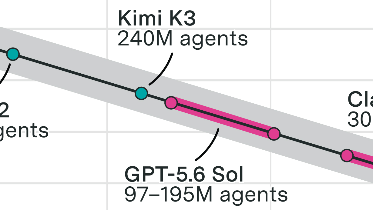
Inference performance improvements can be much larger than changes in raw compute speed (FLOP/s) suggest. We estimate that the Nvidia GB300 provides about 25× Nvidia H100’s inference capacity per chip on the agentic inference workloads we model, with only 2.5× the 8-bit FLOP per second. Comparing FLOP/s alone would therefore underestimate GB300’s inference capacity relative to H100 by a factor of ten. This is because memory and inter-chip communication can matter more than arithmetic throughput for inference performance.
We introduce the Inference Performance Index (IPI) to capture these differences. The index compares how many requests each chip can serve at once across a range of required output speeds. IPI Version 1 focuses on agentic workloads and combines results across four representative models.
Scores are expressed in GB300 equivalents (GB300e), with GB300 scoring one by definition.1 A score of two means we estimate that a chip can serve twice as many users or agents at once as GB300, on average across the workloads and output-speed requirements in the index. We use GB300 as our reference because it is a widely used inference GPU with leading benchmark performance, such as in SemiAnalysis InferenceX.
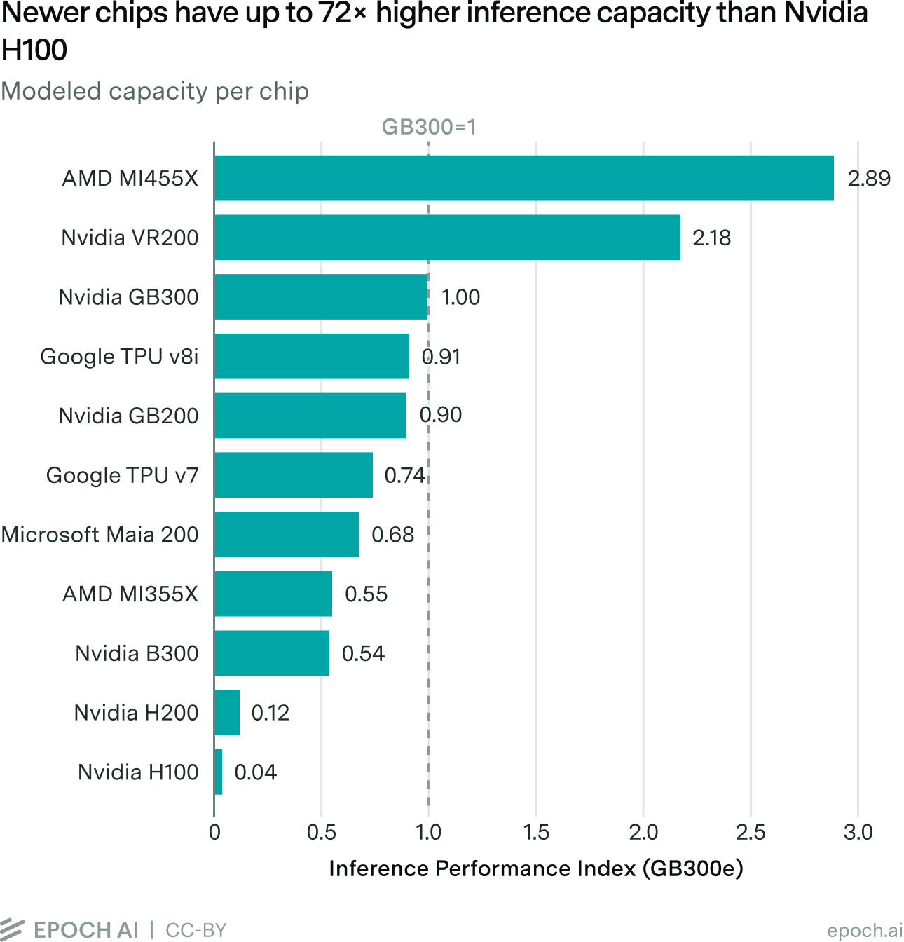
System configuration also matters. Nvidia GB300 NVL72 has about 1.9× the modeled inference capacity per GPU of Nvidia B300 HGX. Both use Blackwell Ultra GPUs, but GB300 connects groups of 72 GPUs through high-bandwidth links, compared with groups of eight for B300 HGX.
The IPI provides a common unit, GB300 equivalents, to estimate a data center’s total inference capacity, or even the world’s. Combined with performance estimates for a particular model and output-speed requirement, this gives a rough estimate of how many users or agents that hardware could serve simultaneously.
This report explains how the index works and the key choices behind it. The accompanying technical methodology provides the equations, assumptions, and implementation details.
The tradeoff between concurrency and output speed
Language model inference has two phases. Prefill, also called the context phase, processes the input and stores intermediate representations in a cache, usually a key-value (KV) cache.2 Decode, or generation, produces the response through repeated forward passes. Each pass processes the latest token using the cached context, updates the cache, and generates one new token per request.3
To illustrate how the cache grows across requests, suppose a coding agent makes a request to the model with 200,000 tokens of cached history and 1,000 tokens of new input consisting of code-search results. Only the new input needs prefill. During decode, the model generates 1,000 output tokens, including reasoning and a tool call to read a different file. The software running the agent executes the tool call and includes the file’s contents as new input in the next request to the model. That request can reuse about 202,000 tokens of cached history: the original 200,000 tokens plus the new input and output from the previous request. Only the new input from the file needs prefill. The cache still occupies memory and is accessed during both prefill and decode.4
During decode, the system can process requests together in a batch. Model weights are stored in high-bandwidth memory (HBM) and brought into faster on-chip memory as needed for computation. Each forward pass processes the model layer by layer, reusing the weights brought on-chip across the requests in the batch. This amortizes the cost of reading weights from HBM. Each additional request still adds cache reads and other request-dependent work, so larger batches can increase total throughput while slowing token generation for each request, even when performance remains memory-bandwidth-bound.
There’s a tradeoff between concurrency and output speed. Concurrency is the number of requests being served simultaneously, expressed in requests per chip. Output speed, in tokens per second per request (tokens/s/req), measures how quickly each request generates tokens. Throughput, in tokens per second per chip (tokens/s/chip), measures the chip’s total output.
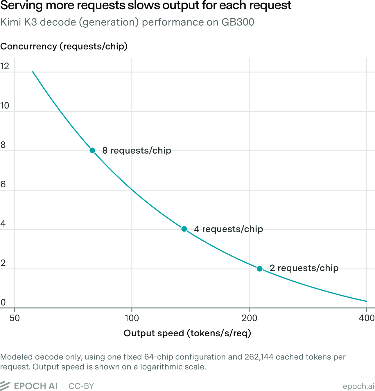
Increasing concurrency from two to eight requests/chip lowers output speed from about 210 to 80 tokens/s/req.
Throughput equals concurrency multiplied by output speed. Using these rounded values, throughput rises from 2 × 210 = 420 to 8 × 80 = 640 tokens/s/chip, an increase of roughly 50% despite slower generation for each request.
The IPI accounts for this tradeoff by comparing how many simultaneous requests each chip can support across a range of output speeds.
How we calculate the IPI
We use Nvidia’s AISimulate to estimate inference performance from the operations required by each model and the following hardware inputs:
- Arithmetic throughput: dense floating-point operations per second per chip, separately for BF16, FP8, and FP4, with the supported precision specified for each accelerator.5
- Memory capacity: HBM bytes per chip, which limit how many model weights and request caches fit.
- Memory bandwidth: HBM bytes transferred per second per chip.
- Interconnect bandwidth: one-way outbound bytes per second per chip at each modeled communication tier, within and between connected groups of chips.
- Interconnect grouping and latency: the number of chips in each communication domain and the assumed communication latency and topology adjustments.
The resulting performance estimates are analytical projections of optimal performance under the modeled hardware limits, often called speed of light (SOL).
The IPI includes both prefill and decode performance. We model them separately, and provision enough prefill chips to avoid bottlenecking decode. We then divide the number of simultaneous requests by the total number of prefill and decode chips to obtain capacity in requests/chip.
The IPI aims to track a representative basket of important inference workloads. Version 1 focuses on agentic inference, which already dominates token usage on OpenRouter, a platform that routes developer requests across AI model providers. In late September 2026, agentic API keys consumed roughly seven times as many tokens as human API keys.
Our agentic workload combines a long cached context of 262,144 tokens with 1,024 new tokens per prefill. To determine the required prefill resources, we use a trace-derived ratio of approximately 1.51 new input tokens per generated output token. The calculation also includes speculative decoding.6 The workload documentation gives the full assumptions.
For each chip and model, we take the highest concurrency per chip achievable at each required output speed across the configurations we evaluate. These points form the capacity curve.
Comparing capacity across output speeds
A chip’s advantage over another can vary with the required output speed. We therefore compare capacity over 50–400 tokens/s/req.
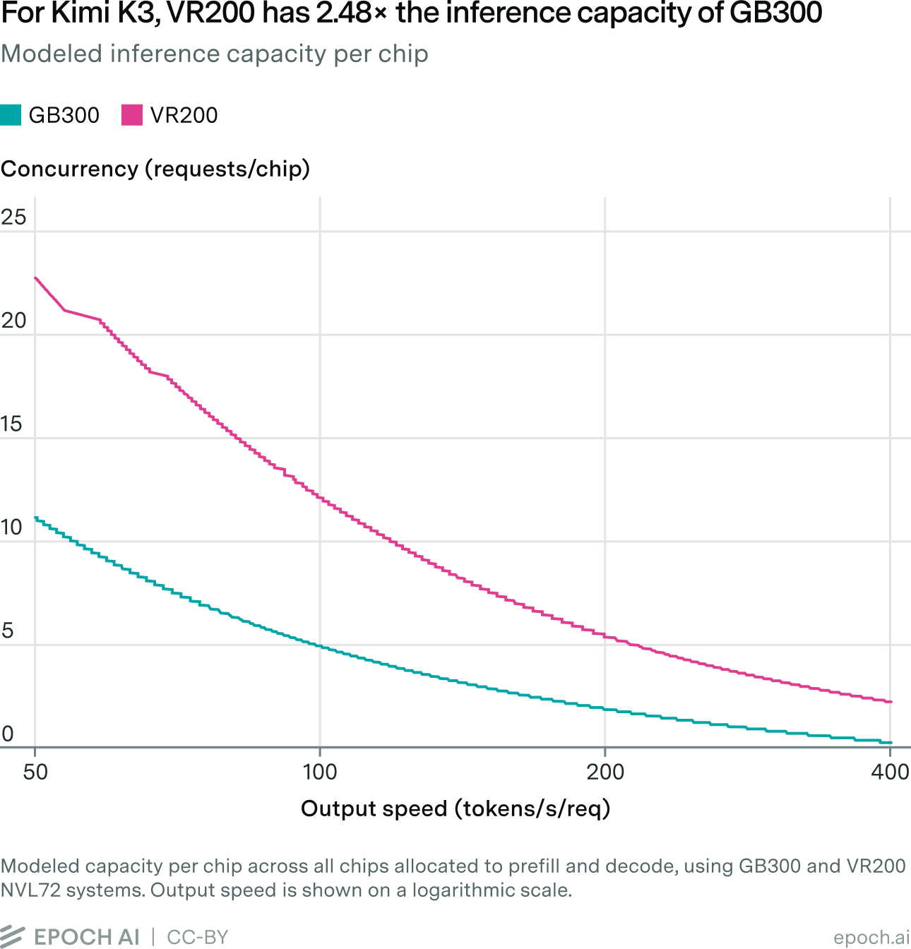
We calculate the area under each curve using a logarithmic output-speed axis. This gives equal weight to each doubling of the required speed: 50–100, 100–200, and 200–400 tokens/s/req.
We divide the area under each chip’s capacity curve by GB300’s for the same model. For Kimi K3, this ratio is approximately 2.48 on the Vera Rubin (VR200) chip, though its advantage varies with the required output speed.
Relative inference capacity for Kimi K3
\[\frac{\text{Area under VR200’s curve}}{\text{Area under GB300’s curve}} \approx 2.48\]Combining the model comparisons
We select four representative architectures that we can accurately model using AISimulate, including a proxy for MAI-Base-2. Attention architectures differ in both the cache stored per request and the data read during decoding.7 For each model, we express the chip’s capacity relative to GB300, then take a simple average of the four ratios to obtain its IPI score.8
IPI score of a chip
\[\text{IPI score} = \frac{1}{4} \sum_{m=1}^{4} \frac{\text{Area under the chip’s curve for model } m}{\text{Area under GB300’s curve for model } m}\]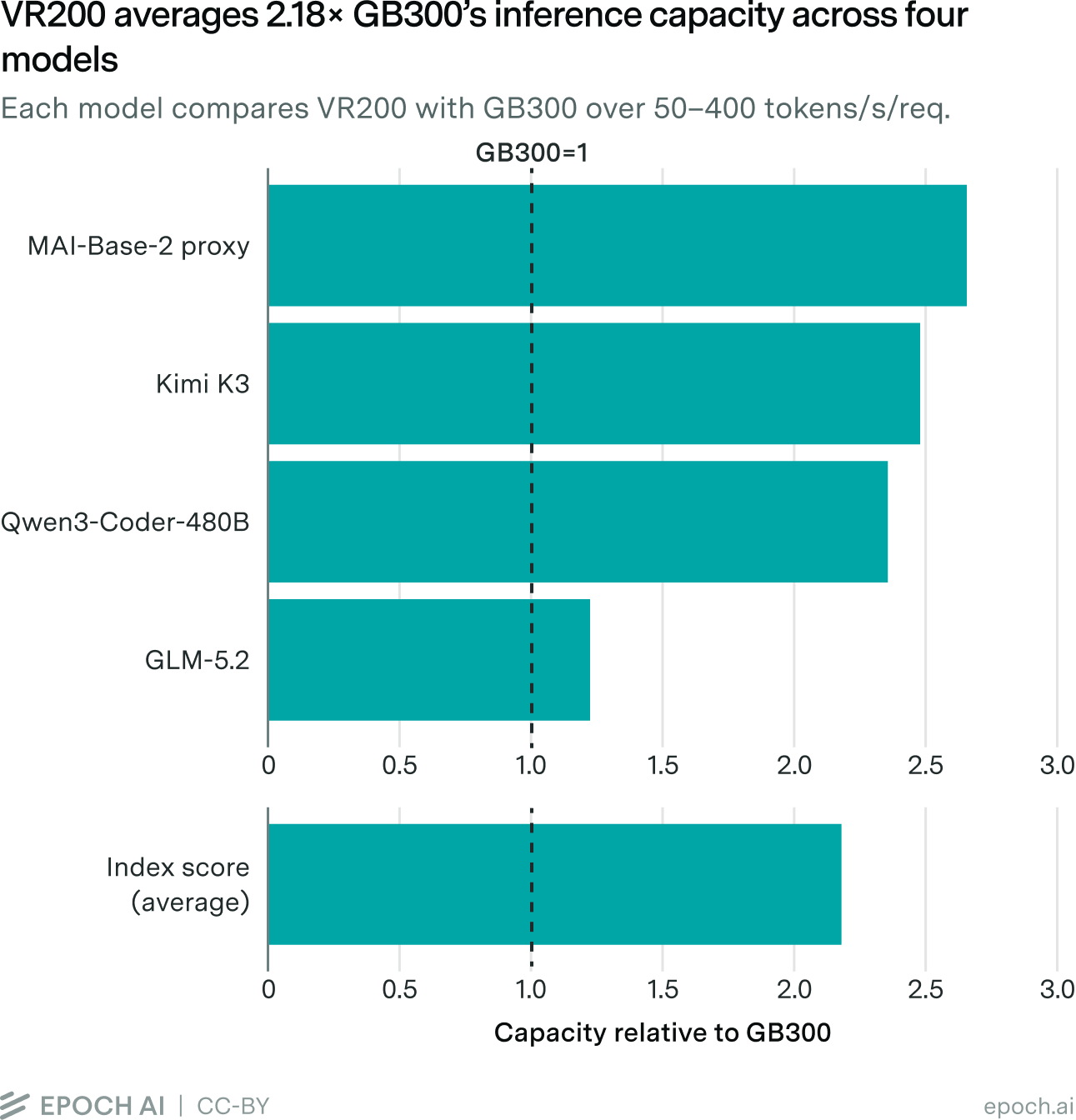
The accompanying sensitivity analysis examines how scores change with the model selection, output-speed range, weighting, and prefill requirements.
Interpreting the IPI
GB300 NVL72 scores 1 GB300e, compared with 0.12 for H200 HGX, a roughly eightfold increase in modeled capacity per GPU. Within Blackwell Ultra, GB300 NVL72 scores about 1.9× B300 HGX (0.54), highlighting the importance of its larger scale-up domain. MI355X scores about 0.55, while VR200 scores 2.18. We can also express a fleet’s capacity in GB300 equivalents.
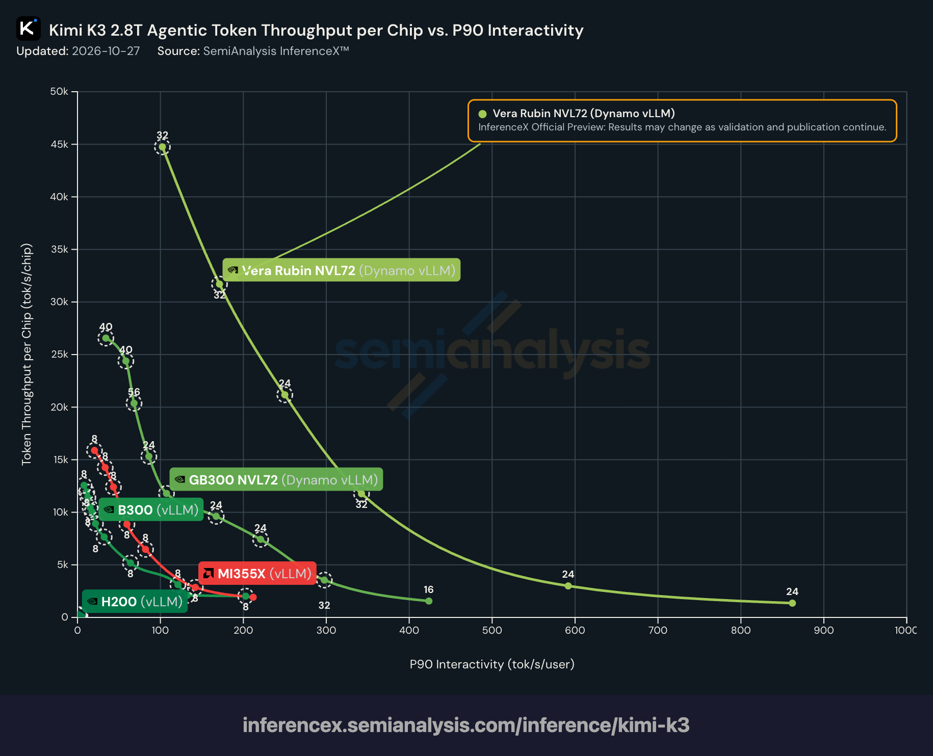
InferenceX’s Kimi K3 benchmarks show a similar ordering, with Rubin and GB300 ahead of B300 and MI355X, and H200 far behind.9
Source: SemiAnalysis InferenceX.
For Kimi K3 alone, our model predicts roughly a 46-fold GB300 advantage over H200, compared with eightfold across the full basket. InferenceX also attributes part of Hopper’s weak Kimi K3 performance to missing software optimizations.
Future versions of the IPI will update the workload and model selection as inference demand changes. We plan to add important new open models when we can accurately model their architectures using AISimulate. Hardware comparisons should use scores from the same IPI version, since changing the basket can change a chip’s score even when its hardware is unchanged.
To learn more, visit the Machine Learning Hardware data explorer to find the methodology, full dataset, interactive visualizations, and more analysis.
Acknowledgements
Special thanks to Eleonora Dello Iacono for designing the figures and thumbnail, and to Cathy Bogaart for editing.
-
These scores describe modeled hardware potential. They do not account for differences in software maturity, which affect how much of that potential is realized in practice. We expect AI-assisted software optimization to help narrow this gap over time.

-
We use “cache” to include different forms of retained model state. In Kimi K3, full-attention layers retain a KV cache that grows with context length, while linear-attention layers retain a fixed-size recurrent state.
-
This describes standard autoregressive decoding. With speculative decoding, the target model verifies several proposed tokens in one forward pass, so a pass can produce multiple accepted output tokens. Producing the proposed tokens requires additional work, which our calculation also includes.
-
For a visual example, see Figure 1 in vLLM’s analysis of Codex traces on SWE-bench Pro, which shows cached history accumulating as each request adds new input and output tokens. See also the diagram in SemiAnalysis’s overview of agentic workloads.
-
We use different numerical precisions for different accelerators and model operations. We have not established that these choices preserve equivalent model quality. See the methodology documentation.
-
Our calculation assumes an average of three accepted output tokens per decoding cycle. This acceptance length is a modeling assumption, not a measured acceptance rate for every model. See the execution-time assumptions.
-
The models differ in how much context they store and read. GLM-5.2 retains a compressed cache of the full context, but its main attention operation reads selected tokens. Kimi K3 combines linear and full attention, while Qwen3-Coder-480B uses full-context grouped-query attention. Our MAI-Base-2 proxy combines sliding-window and global attention. These differences affect memory use per request and the data read during decoding. See the methodology for architecture details and proxy assumptions.
-
An arithmetic mean preserves a chip’s contribution on models it serves well. A geometric mean penalizes uneven performance more strongly, substantially lowering Hopper’s scores, but makes comparisons independent of the reference chip.
-
In our validation study, GB300’s measured Kimi K3 throughput closely tracked predictions assuming 50% of modeled SOL performance, with an average absolute difference of about 12% across five frontier points at 50–400 tokens/s/req.
About the authors
Related work