Overview
AI companies are spending hundreds of billions of dollars a year on chips and data centers, on the premise that those chips will run AI agents to do work that people do today. How many agents could this hardware buildout actually support?
- AI chips shipped through 2027 could run tens to hundreds of millions of concurrent frontier-model agents. Running nonstop, these agents would supply as many weekly working hours as about 140–720 million full-time employees.
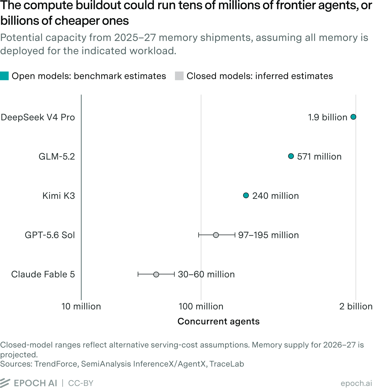
- More efficient models could potentially support billions of agents on the same hardware. Applying DeepSeek V4 Pro serving benchmarks to the projected hardware supply yields approximately 1.9 billion concurrent agents supplying as many weekly working hours as 8 billion people each working 40 hours.
- Even modest use of this capacity would require a massive increase in global demand for AI. Using 20% of our central capacity estimate would imply $2.6–5.3 trillion a year in API-equivalent spending, against roughly $1 trillion in developer revenue by end-2027 at fivefold annual growth.
- Hourly agent spending varies substantially across models and harnesses. In our analysis of agent traces, Codex workloads averaged roughly $16–18 per hour of continuous agent activity, compared with $24–50 for Claude Code workloads.
Potential agent capacity and spending
Anthropic’s Dario Amodei has described a future “country of geniuses in a datacenter”, but how many AI agents could future data centers actually support? That scale matters for AI’s potential impact on the economy and labor force.
We find that hardware using high-bandwidth memory (HBM) shipped during 2025–27 could eventually support tens to hundreds of millions of concurrent frontier-model agents, assuming full deployment and allocation to these workloads. HBM shipped during 2025–26 could support 16–56 million concurrent agents once deployed. Including shipments through 2027 raises that estimate to about 30–170 million.1
But unlike humans, an AI agent can work all 168 hours each week, 4.2 times the 40-hour workweek for a full-time employee. Therefore, these agents could work as many weekly hours as about 67–240 million people from hardware shipments through 2026, and about 140–720 million from shipments through 2027. For scale, the United States has a population of 342 million and an estimated 100 million knowledge workers. These comparisons count working hours alone. Agents can also produce output much faster than humans, though the quality of that output varies.
Even if we use only 20% of the capacity from memory shipped through 2027, the implied spending at API prices would be $2.6–5.3 trillion a year once the hardware is deployed.2 For comparison, if model developers’ revenues keep growing fivefold each year, their combined annualized revenue would reach roughly $1 trillion by the end of 2027.
Demand could fall behind this potential supply, creating an overabundance of capacity. The key uncertainty is whether sustained, rapid growth in demand for AI services will justify the investment.
How we estimate agent capacity
We estimate potential concurrent agents (\(A\)): how many agents could run at once on the memory shipped during 2025–27, assuming full deployment and allocation to the modeled workload. We use these capacity estimates to derive working-hour and API-equivalent spending figures under the stated operating-time, pricing, allocation, and utilization assumptions.
Our estimate of potential concurrent agents is built from two terms:
\[\begin{aligned} A &= E \times c, \\[6pt] \text{where}\quad A &= \text{potential concurrent agents}, \\ E &= \text{effective hardware supply in GB300 equivalents}, \\ c &= \text{agents per GB300 equivalent}. \end{aligned}\]Effective hardware supply (\(E\)): measured in GB300-equivalent inference units, analogous to FLOP-based H100 equivalents. For these workloads, memory capacity constrains concurrency and memory bandwidth constrains streaming speed. We count high-bandwidth memory (HBM) shipped from 2025 onward, including HBM3E and newer generations, in units of 288 GB, matching a GB300 GPU. We then adjust for the concurrency that newer hardware can support:
\[E = \frac{H_3 + u \times H_4}{288},\]where \(H_3\) and \(H_4\) are cumulative HBM3E and HBM4/4E supply (GB). \(u\) is the ratio of agent sessions per GB on HBM4/4E systems to agent sessions per GB on HBM3E systems.
Serving capacity (\(c\)): concurrent active agent sessions per GB300 equivalent.
We use
\[c = \frac{G \times K}{S}\]for closed models. \(S\) is API spending per active agent-hour ($/agent-hour), using durations adjusted to remove identified human waits and cap other idle gaps. \(G\) is GPU rental cost ($/GB300-hour). \(K\) is API-equivalent revenue divided by reference serving cost.
For open models, we use benchmarked concurrency.
Main assumptions: \(S = \$30/\text{agent-hour}\), \(G = \$5/\text{GB300-hour}\), \({K = 5\text{–}10\times}\), and \({u = 2\times}\). We also test \({u = 1\times}\) and \(4\times\).
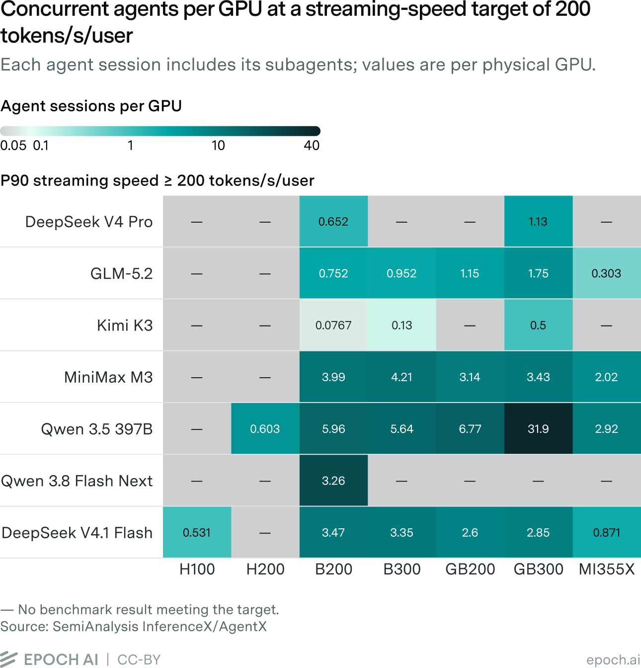
Open-model benchmarks use P90 streaming-speed targets of 50 and 100 output tokens per second per user, with 200 as a sensitivity. We hold current model and workload requirements fixed.
Estimating agent sessions per GPU today
What counts as an agent?
We use “agent” as shorthand for an agentic workload running within a harness such as Codex or Claude Code. An agent session includes model calls and tool use, rather than continuous token generation.
We draw on two sources: SemiAnalysis’s AgentX serving benchmark for open models, and TraceLab, a public dataset of logged agent sessions, for closed models. AgentX counts a main agent and its subagents as one session tree; TraceLab’s accounting groups do not always capture that complete tree. We use “agent” and “agent session” interchangeably when discussing capacity. A continuous agent session includes the time spent waiting for tool calls. We estimate the continuous working time by removing time spent waiting for human input and also capping unidentified idle time. One hour of this adjusted activity counts as one agent-hour.
For open models, serving benchmarks directly measure how many concurrent agent sessions the hardware supports at a given output speed. For closed models, we estimate concurrency from hourly spending and serving-cost assumptions.
Open models: serving benchmarks measure concurrency directly
For open models, we use the benchmark data from SemiAnalysis’s InferenceX AgentX. The AgentX benchmark uses a dataset of Claude Code agent session traces collected by SemiAnalysis. The benchmark replay uses synthetic text while preserving request lengths, shared context, and the timing and structure of model calls. Further details in the AgentX methodology.
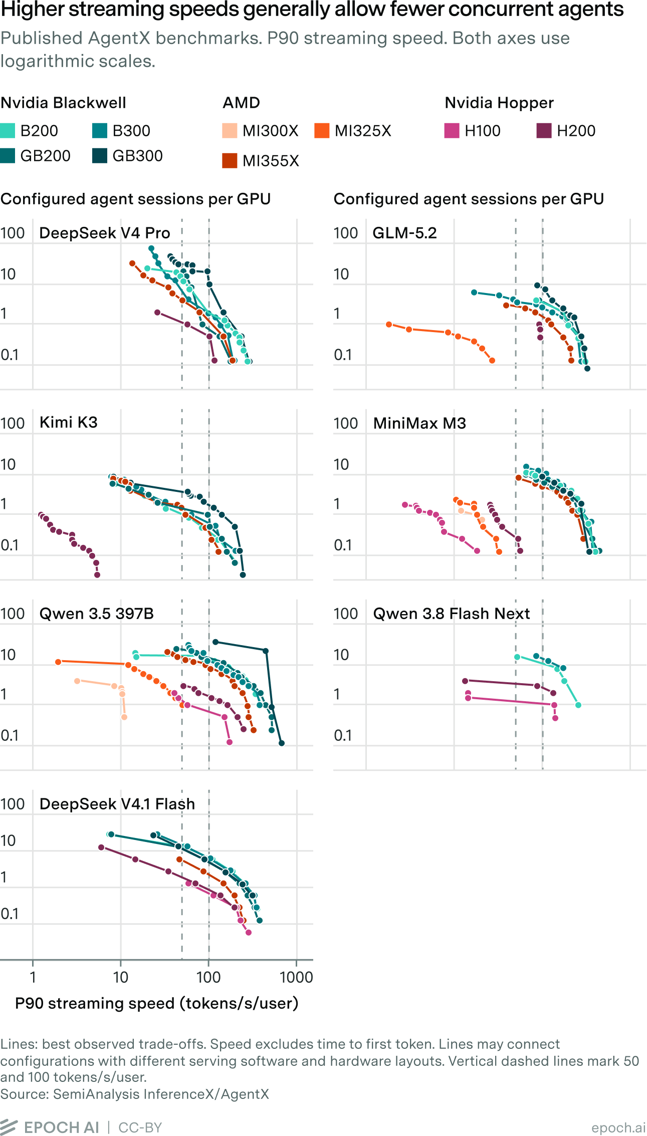
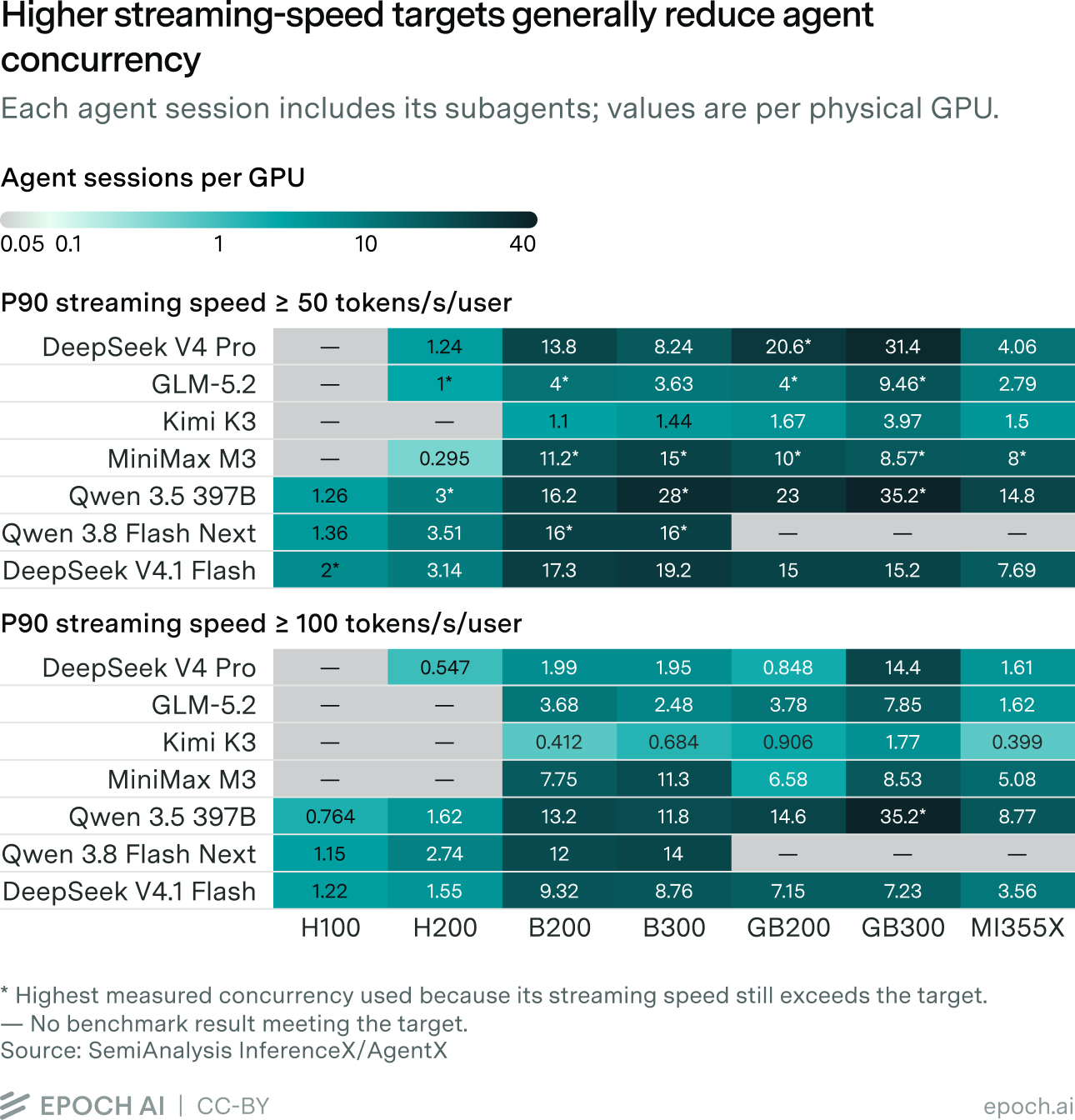
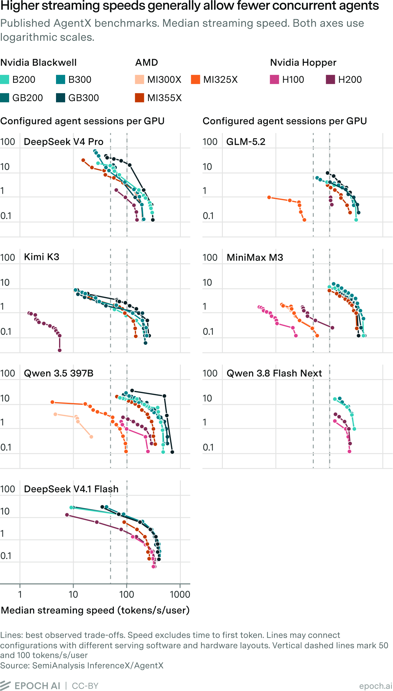
Concurrency for AgentX is defined by the number of agent sessions launched. We divide the concurrency by the total number of GPUs to derive a metric of concurrent agent sessions per GPU. For prefill-decode disaggregated configurations, we count the number of combined GPUs. Figures 2–3 show the published configurations and the agent sessions per GPU.
Speed targets: 50 and 100 tokens per second per user
We use 50 and 100 TPS/user as round reference points for output speed in tokens per second. 200 TPS/user is also given in the appendix to test a more demanding scenario. For reference, both OpenAI and Anthropic tend to serve their frontier models around 50–70 TPS. In the benchmark data, P90 interactivity describes the output speed in TPS/user for the slower end of the distribution. This excludes the time to first token (TTFT) and does not measure end-to-end latency (see Appendix A).
The figures use the AgentX snapshot dated in Table 2 and cover seven models. We excluded any preview data not run directly through the InferenceX public repo.
Concurrency per GPU at the main speed targets
Closed frontier models: concurrency inferred from API spending
Since closed frontier models lack the architecture details needed for transparent hardware benchmarks, we instead look at the API costs of a continuously running agent. We analyzed TraceLab’s dataset of Codex and Claude Code agent sessions. We adjusted for human delays (agent waiting on human response) and divided spending by agent working time to normalize to an hourly rate. Using the API prices listed in Table A3, we calculated the API-equivalent spending per agent-hour.
We then estimate how much of that spending covers serving costs, using an assumed markup ratio of API revenue to serving cost. Comparing the resulting cost per agent-hour with the rental cost of a GB300 GPU gives an estimate of how many concurrent agents each GPU could support.
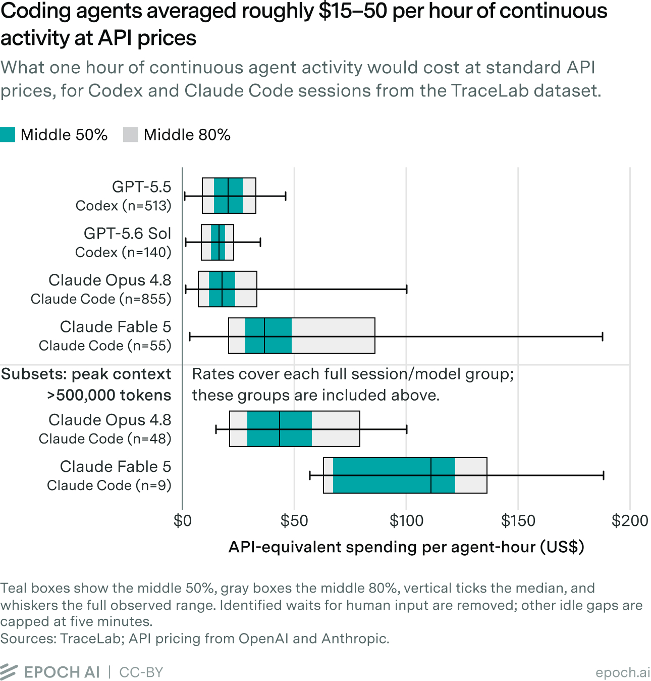
$30 per agent-hour sits between Codex and Claude Code costs
Hourly spending varies across models and harnesses. Under Figure 4’s retained-cache4 and five-minute gap-cap assumptions, TraceLab’s pooled rates are $18.2/hour for GPT-5.5, $15.5 for GPT-5.6 Sol, $24.3 for Opus 4.8, and $50.2 for Fable 5. We choose $30/hour as a round reference point which sits slightly towards the higher end. Future models may go up in price as with the jumps to Fable for Anthropic and GPT-6 Astra for OpenAI or they may go down due to competition and efficiency improvements. Figure 8 goes through a range of prices from $10 to $100 per agent-hour.
Let \(S\) be API spending per agent-hour and \(K\) the ratio of API-equivalent revenue to serving cost at our reference GPU rental price. \({K = 10\times}\) means $10 of API billing for every $1 of that cost.
The implied serving cost per agent-hour is \(S/K\). Dividing the GPU-hour rental price, \(G\), by this cost gives agent sessions per GB300 equivalent:
\[\begin{aligned} \text{agent sessions per GB300 equivalent} &= \frac{G}{S/K} \\[4pt] &= \frac{G \times K}{S}. \end{aligned}\]Table 1 uses \(S = \$30\) per agent-hour and \(G\) = $5.00/GB300-hour, from SemiAnalysis’s Rent – 3 Year Commit tier. At \({K = 10\times}\), the implied serving cost is $3 per agent-hour. A $5 GPU-hour supports 1.67 concurrent agent sessions.
| Revenue/cost \(K\) | Implied cost/agent-hour | Agents/GB300 equiv. |
|---|---|---|
| 5× | $6.00 | 0.833 |
| 10× | $3.00 | 1.667 |
Table 1. Closed-model assumptions at $30 per agent-hour and $5 per GB300-hour. Appendix B tests higher revenue/cost multiples.
Our main case uses \({K = 5\text{–}10\times}\), giving 0.833–1.667 agent sessions per GB300 at $30 per agent-hour. Table 2 shows the ratio \(K\) at around 4–10× for open models on AgentX at 50 TPS/user.5
Open-model benchmarks imply revenue/cost ratios of 2–10×
We compare the assumed multiples with what each open-model benchmark would earn at its model’s API rates, using theoretical cache-hit rates. At each P90 speed target, we select the GPU with the lowest three-year rental cost per concurrent agent-hour.
Each speed column reports \(K\), the ratio of API-equivalent revenue to GPU rental cost. The GPU with the lowest rental cost per agent session need not have the highest \(K\).
InferenceX reports how much input could theoretically reuse a prefix. We price those tokens at the model’s cached-input rate and the rest at its ordinary input rate. Actual API billing could be higher or lower if the provider caches a different share.
| Model / API tier | GPU | 50 TPS/user | 100 TPS/user |
|---|---|---|---|
| DeepSeek V4 Pro off-peak | GB300 | 4.4× | 2.1× |
| DeepSeek V4 Pro peak | GB300 | 8.8× | 4.2× |
| GLM-5.2 | GB300 | 10.5× | 9.3× |
| Kimi K3 | GB300 | 4.1× | 2.9× |
| MiniMax M3 | B300 | 4.8× | 4.1× |
Table 2. API-equivalent revenue divided by GPU rental cost at the selected 50 and 100 TPS/user configurations for select open models from AgentX. MiniMax uses the short-context token pricing.6
We use the same SemiAnalysis reported rental rates, $5.00/GB300-hour and $4.25/B300-hour, to calculate \(K\) for GPUs running the AgentX benchmark. We price theoretical cache reuse at each frontier endpoint, and interpolate to get concurrency and API-equivalent revenue per GPU-hour at the desired TPS/user. Where the frontier stays above a speed target, we use its highest observed concurrency.
The AgentX and TraceLab workloads are comparable
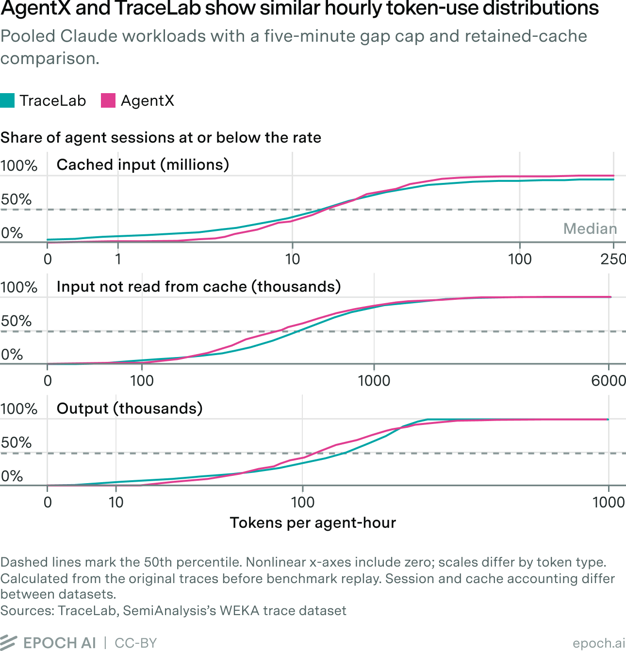
AgentX replays Claude Code session trees from the WEKA corpus. Due to differences in the format of the AgentX WEKA traces compared to TraceLab traces, we plotted a comparison between the common Claude models of both to check that the workloads are similar enough to be comparable. Figure 5 compares their hourly token consumption broken down by token type after processing.
Estimating future capacity from high-bandwidth memory
HBM is the common bottleneck across AI accelerators
HBM gives us a common measure of supply across GPUs and custom AI accelerators because it is simultaneously an important component for inference and a main bottleneck for chip production. The primary producers of HBM are just three companies: Micron, Samsung, and SK hynix. Micron reports that memory demand exceeds supply and new fabs take years to build, while SK hynix also reports demand above its supply capacity. Nvidia is also reported to be evaluating lower-memory configurations for Rubin Ultra due to these supply constraints.
HBM capacity constrains how many requests can stay active at once. Memory must hold model weights and the KV cache, which grows with context length for each request. Longer contexts require more cache space. HBM bandwidth can constrain the decode speed in terms of TPS/user when the bottleneck is the time to stream the weights and KV cache from memory.
We count physical HBM capacity in units of 288 GB, matching the GB300-class GPU used in our benchmarks.8 This provides a common memory unit across vendors. We then adjust for the performance of newer systems to express supply in effective GB300 equivalents.9
| Accelerator | HBM generation | Memory per GPU | Peak bandwidth per GPU |
|---|---|---|---|
| A100 80GB SXM | HBM2E | 80 GB | 2.039 TB/s |
| H100 SXM | HBM3 | 80 GB | 3.35 TB/s |
| Blackwell Ultra (GB300) | HBM3E | 288 GB | 8 TB/s |
| Rubin (VR200) | HBM4 | 288 GB | 22 TB/s |
Table 3. Published memory specifications for representative GPUs. Values are per GPU. Appendix C lists capacity and bandwidth specifications for individual HBM stacks.
Newer HBM4 systems should support more agents per gigabyte
Nvidia’s Blackwell Ultra and Rubin specifications show that GB300 uses 288 GB of HBM3E while VR200 uses 288 GB of HBM4. While capacity has remained fixed, this change in HBM generation moves the bandwidth from 8 to 22 TB/s (a 2.75× increase).
When memory capacity is the constraint, concurrency is capped by the maximum number of requests that can fit in memory. More bandwidth can support more agents at a given output speed when bandwidth is the bottleneck.10
Our central assumption is that HBM4/4E systems support twice as many concurrent agents per 288 GB as HBM3E systems (\(u = 2\)). The gain depends on the workload and its bottlenecks, so we also test no improvement (\(u = 1\)) and a fourfold improvement (\(u = 4\)). The fourfold case allows for gains beyond memory bandwidth, such as better interconnects and more efficient serving software.
We count all HBM3E and newer memory shipped since 2025
These shipment years identify the hardware included in each estimate; deployment follows later. Epoch’s AI Chip Components methodology assumes roughly eight weeks from HBM entering accelerator packaging to completion of the accelerator, including final assembly and testing. Time to deployment can be significantly longer and much less predictable when it depends on data center construction.
We reconstruct annual supply from public TrendForce releases: 2026 HBM shipments above 3.75 billion GB, 2026 HBM usage growth above 70%, and projected 2027 shipment growth of 50–60%. Table 4 uses the first two thresholds as point estimates and the midpoint of the 2027 growth range.11 The following are our derived estimates. See Appendix B for detailed calculations.
| Shipment year | Total HBM B GB | HBM3E share | HBM4/4E share |
|---|---|---|---|
| 2025 | 2.21 | 80% | 0% |
| 2026E | 3.75 | 62.5% | 37.5% |
| 2027E | 5.81 | 20% | 80% |
Table 4. Annual HBM shipments in billions of GB and estimated generation shares. The 2026–27 shares are assumptions.
Assumptions made:
- For 2025, TrendForce expects more than 80% of HBM bit demand to be HBM3E. We use 80% and exclude the remaining 20% as older HBM.
- TrendForce expects HBM4 to overtake HBM3E in the second half of 2026 but gives no full-year share. We assume HBM4 accounts for 37.5% of annual shipments.
- For 2027, TrendForce identifies HBM4 as the mainstream generation. We assume HBM4/4E accounts for 80% of shipments, with the remainder HBM3E.
Shipments through 2027 could support 33–171 million frontier-model agents
We calculate total concurrent agents in two steps:
\[\begin{aligned} E &= \frac{H_3 + u \times H_4}{288} \\[6pt] A &= E \times c \end{aligned}\]\(H_3\) and \(H_4\) are cumulative HBM3E and HBM4/4E supply in GB. Weighting \(H_4\) by \(u\) and dividing by 288 gives effective GB300 equivalents, \(E\). Multiplying \(E\) by agent sessions per equivalent \(c\) gives potential concurrency.
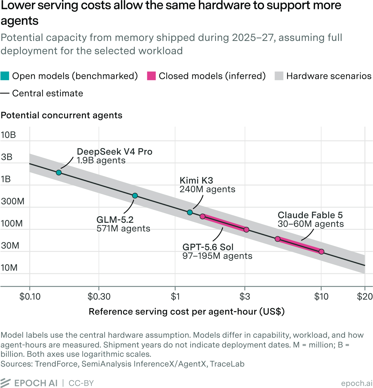
Figure 7 uses the main closed-model estimate of 0.833–1.667 agent sessions per GB300 equivalent, based on \(S = \$30\)/hour, \(G = \$5\)/GPU-hour, and \({K = 5\text{–}10\times}\). It assumes full deployment and allocation to the workload.
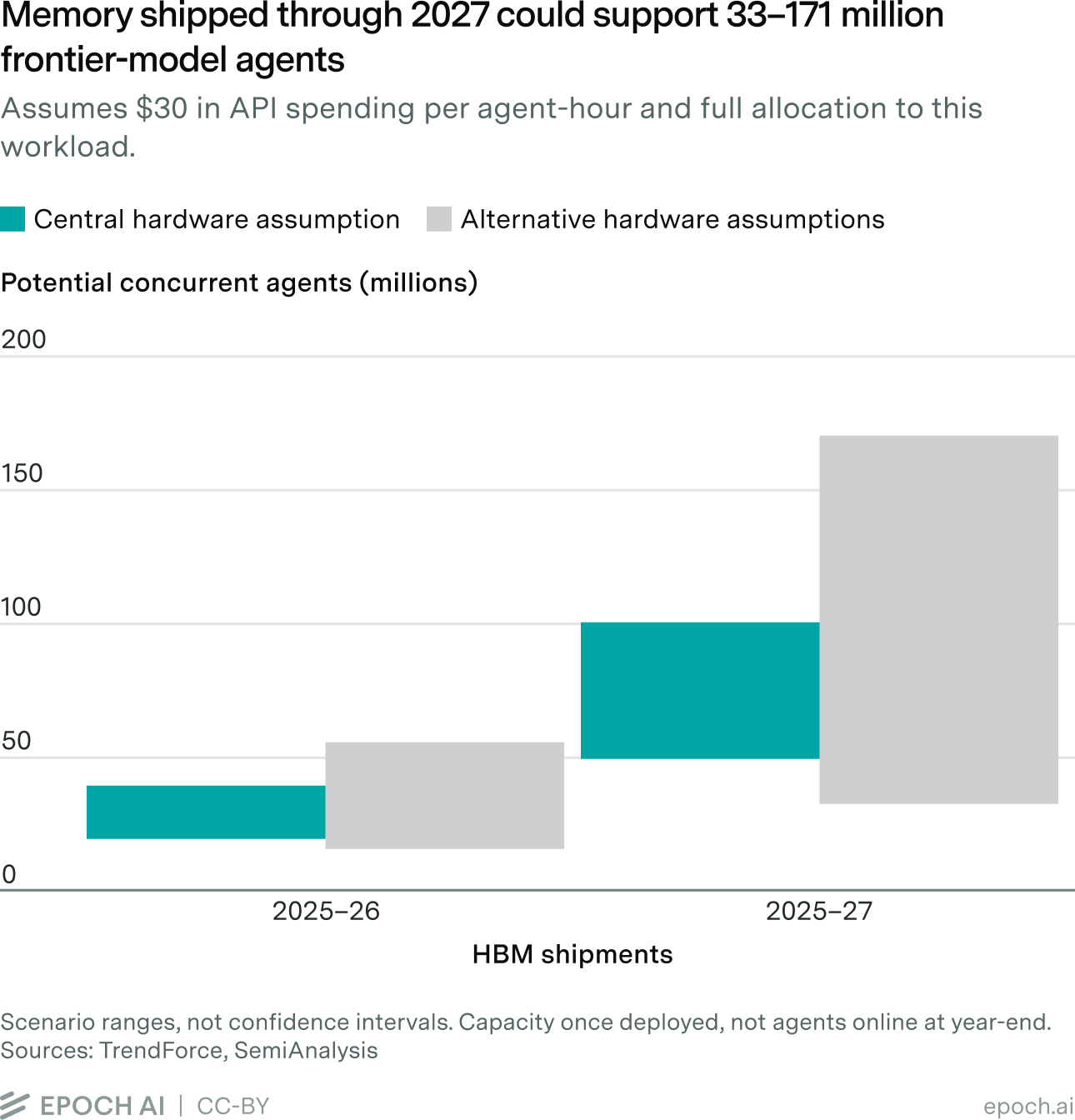
Under the central hardware assumption, shipments through 2026 support approximately 20–40 million concurrent agents, rising to 50–101 million with shipments through 2027. Allocating half the memory to the workload would halve these counts. Appendix B gives results for each hardware assumption.
The 2027 total includes the 2026 total. Each model scenario represents an alternative use of the same hardware pool.
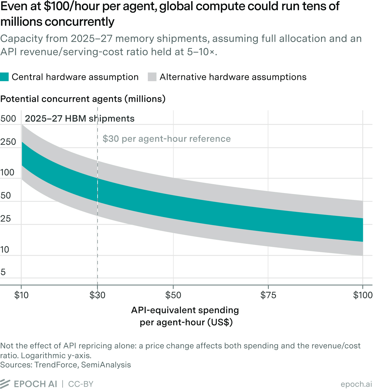
Capacity falls in proportion to spending per agent-hour
Figure 8 shows the change in agents with agent-hour cost varying from $10 to $100 beyond the original $30 central estimate. The bands also show the ranges depending on markup ratio \({K = 5\text{–}10\times}\) and HBM4 uplift \({u = 1\text{–}4\times}\). This shows how the number of total agents drops with higher agent-hour cost. Appendix B gives the numerical grid.
Capacity from open-model benchmarks
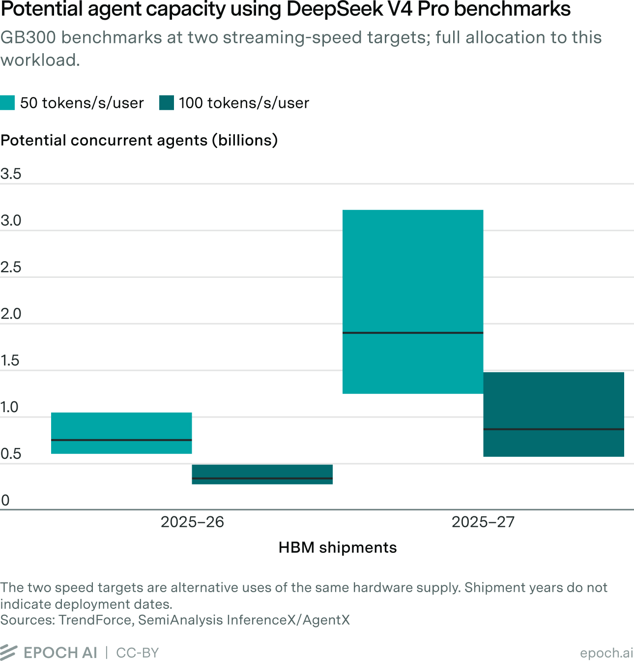
For DeepSeek, the InferenceX GB300 frontier gives 31.4 agent sessions per GPU at 50 TPS/user and 14.4 at 100 TPS/user, including interpolation. We scale these benchmark estimates by effective hardware supply and vary \(u\) from 1× to 4×. See Appendix B for the numerical table containing other open models.
Conclusion: what the totals imply for AI demand
Across our hardware and serving-cost scenarios, memory shipped during 2025–27 could support about 30–170 million concurrent frontier-model agents once deployed and fully allocated to these workloads, supplying as many weekly working hours as about 140–720 million full-time employees. The question this raises is whether demand will be large enough to put this capacity to use.
To compare this capacity with the scale of the inference market, we consider a scenario with conservative use of the available hardware: 40% allocation to revenue-generating inference and 50% utilization, giving 20% effective use of total capacity. Once deployed, hardware using memory shipped during 2025–26 could support approximately $1.1–2.1 trillion in annual API-equivalent spending under our central hardware and reference serving-cost assumptions, rising to $2.6–5.3 trillion when including shipments through 2027, at $30 per agent-hour.13
For comparison, leading model developers already generate over $100 billion in combined annualized revenue. Continuing the recent fivefold annual growth rate would bring this to roughly $1 trillion by the end of 2027, still significantly below the spending implied by our capacity scenario.14
Near-term shortages of serving capacity can coexist with this potential supply. In late 2025, Satya Nadella said Microsoft had chips sitting in inventory that it could not plug in because suitable powered data center space was unavailable. Deployment delays give demand more time to grow. As these bottlenecks ease, accumulated hardware can come online alongside new shipments.
The price of achieving a given level of AI performance is falling rapidly. Epoch’s recent analysis estimates a decline of 47% per quarter since 2023 across the benchmarks studied. This cuts both ways for the buildout. Lower hardware ownership and operating costs can reduce the revenue needed to justify investment. More efficient models and serving systems, however, reduce the hardware required for each task. Maintaining utilization would require demand for agent activity to grow enough to offset those efficiency gains.15
Demand could grow through broader adoption of agents and their use on harder, more computationally demanding tasks. Persistent agents such as OpenAI’s dots could also increase the amount of work delegated by each user by handling ongoing responsibilities and longer projects. Lower prices would make more of these applications economical. If the resulting growth in activity outpaces improvements in compute efficiency, total inference compute demand would rise despite each task requiring less compute, an instance of Jevons’ paradox.16
These estimates suggest a risk that the compute buildout could run ahead of inference demand. Absorbing this capacity will depend on how much work users delegate, how much compute that work requires, and how much they are willing to pay. At hourly costs comparable to human wages, agents will need to deliver enough value to justify that spending. The buildout is a bet that AI will move beyond answering questions to carrying out economically valuable work across a broad range of industries.
Acknowledgements
Thanks to JS Denain, Jaime Sevilla, Venkat Somala, and Josh You for their helpful feedback. Special thanks to Eleonora Dello Iacono for designing the figures and thumbnail, and to Lynette Bye, Linda Petrini, and Elliot Stewart for editing.
Appendices
Appendix A: Additional benchmark and trace data
Median streaming speed
The 200 TPS/user sensitivity
Streaming speed does not include the first-token wait
| P90 speed target (TPS/user) | P90 time to first token (seconds) |
|---|---|
| 50 | 39.8 |
| 100 | 12.4 |
| 200 | 4.6 |
Table A1. P90 time to first token for the highest-concurrency measured Kimi K3 GB300 configuration meeting each streaming-speed target.
These configurations use different deployments, so the results do not isolate the effect of streaming speed on first-token latency. The main concurrency estimates can also interpolate between measured configurations.
TraceLab sample summary
| Model and harness | Agent sessions (pooled / plotted) | Adjusted hours | Pooled USD/hour |
|---|---|---|---|
| GPT-5.5 · Codex | 1,069 / 513 | 866.4 | $18.19 |
| GPT-5.6 Sol · Codex | 206 / 140 | 319.7 | $15.50 |
| Opus 4.8 · Claude Code | 1,947 / 855 | 1,010.0 | $24.34 |
| Fable 5 · Claude Code | 168 / 55 | 100.8 | $50.16 |
| Opus 4.8 · Claude Code peak >500k subset | 48 / 48 | 302.6 | $38.99 |
| Fable 5 · Claude Code peak >500k subset | 10 / 9 | 41.6 | $104.75 |
Table A2. TraceLab sample underlying Figure 4. Pooled USD/hour is total API-equivalent cost divided by total adjusted hours. The two counts show all included session/model groups and those with at least five primary active minutes, which are used for the plotted distribution. Shorter groups remain in the pooled totals.
The “peak >500k” rows contain groups with at least one eligible request above 500,000 input tokens. Their costs and hours cover the whole group, and these groups are already included in the full-model rows. The four full-model rows contain 3,390 session/model groups from 3,382 source agent sessions; a session can contribute to more than one model’s row.
Source: TraceLab v0.0.2; included activity Apr 23, 2026–Jul 24, 2026 (UTC). We use the same cache, gap-cap and pricing assumptions as Figure 4. Claude API prices were recorded Aug 21, 2026; Codex rates were verified Sep 14, 2026. Groups without usable timing or a model we could price are excluded. Five calls within mixed-model groups could not be priced; their time remains included, but their cost is omitted.
Token prices used
| Model | Input | Cached input | Cache writes | Output |
|---|---|---|---|---|
| GPT-5.5 | $5.00 | $0.50 | — | $30.00 |
| GPT-5.6 Sol | $4.00 | $0.40 | $5.00* | $20.00 |
| Claude Opus 4.8 | $5.00 | $0.50 | $6.25 | $25.00 |
| Claude Fable 5 | $10.00 | $1.00 | $12.50 | $50.00 |
Table A3. Frozen token prices for the four model rows in Figure 4 (US$ per million tokens). Standard API rates; no fast-mode, Batch, Flex, subscription or negotiated discounts. Pricing snapshot dates are given in the source note above.
* GPT-5.6 Sol’s non-read input is assumed to be cache-written at $5/M rather than charged at the $4/M ordinary input rate; this allocation is not observed in the traces. GPT-5.5 has no separate write surcharge in the analysis. Claude write prices are the five-minute cache-write rates.
For GPT requests exceeding 272,000 input-context tokens, input and cache rates are multiplied by 2 and output rates by 1.5. No included GPT-5.5 group exceeds that threshold. The displayed Claude rates have no long-context multiplier. Mixed-model calls retain their own frozen tariffs. Cache-retention and timing adjustments are unchanged.
Appendix B: Capacity calculations and sensitivities
Higher revenue/cost multiples
| Revenue/cost \(K\) | Implied cost/agent-hour | Agents/GB300 equiv. |
|---|---|---|
| 5× | $6.00 | 0.833 |
| 10× | $3.00 | 1.667 |
| 20× | $1.50 | 3.333 |
| 40× | $0.75 | 6.667 |
Table B1. Serving cost and concurrency at \(S = \$30\)/hour and \(G = \$5\)/GPU-hour. The main estimate uses \({K = 5\text{–}10\times}\); the 20× and 40× cases test lower serving costs relative to API revenue.
HBM reconstruction details
| Shipment year | Total HBM B GB | HBM3E share | HBM4/4E share | HBM3E B GB | HBM4/4E B GB |
|---|---|---|---|---|---|
| 2025 | 2.21 | 80% | 0% | 1.76 | 0 |
| 2026E | 3.75 | 62.5% | 37.5% | 2.34 | 1.41 |
| 2027E | 5.81 | 20% | 80% | 1.16 | 4.65 |
Table B2a. Annual HBM supply in billions of GB. Total supply is 3.75 / 1.70 for 2025 and 3.75 × 1.55 for 2027. We exclude the 20% of 2025 supply consisting of older HBM. The 2026–27 generation shares are assumptions. Calculations use unrounded inputs.
We assume HBM4/4E accounts for 37.5% of shipments in 2026 and 80% in 2027, following the transition described in the main text. The sources do not specify these annual shares.
| Shipments through | HBM3E (billion GB) | HBM4/4E (billion GB) | HBM3E 288 GB units (millions) | HBM4/4E 288 GB units (millions) | Effective GB300 equivalents (millions; \(u = 2\)) |
|---|---|---|---|---|---|
| 2026 | 4.108 | 1.406 | 14.27 | 4.88 | 24.03 |
| 2027 | 5.271 | 6.056 | 18.30 | 21.03 | 60.36 |
Table B2b. Cumulative eligible HBM, physical 288 GB memory units, and effective GB300-equivalent supply. The final column adds HBM3E units to twice the HBM4/4E units (\(u = 2\)). Calculations use unrounded inputs.
For shipments through 2026, \(E = (4.10846 + 2 \times 1.40625)\text{ billion GB} / 288\text{ GB} \approx 24.03\) million GB300 equivalents. Multiplying by the main 0.833–1.667 agent sessions per equivalent (Table B1) gives approximately 20–40 million concurrent agents at full allocation.
Capacity by hardware uplift
| Supply through | 1× uplift | 2× uplift central | 4× uplift |
|---|---|---|---|
| 2026 | 16.0–31.9 | 20.0–40.1 | 28.2–56.3 |
| 2027 | 32.8–65.6 | 50.3–100.6 | 85.3–170.7 |
Table B3. Millions of concurrent agents at \(S = \$30\)/hour and \({K = 5\text{–}10\times}\), assuming full deployment and allocation. Both rows count shipments from 2025 onward; the 2027 total includes the 2026 total.
Capacity by hourly spending and model
| Scenario | Agents per GB300 | Through 2026 (Million agents) | Through 2027 (Million agents) |
|---|---|---|---|
| Panel A. Closed models — \({K = 5\text{–}10\times}\); \({u = 1\text{–}4\times}\) | |||
| Closed-model $2.5/hour | 10.0–20.0 | 191.5–675.9 | 393.3–2,048.3 |
| Closed-model $5/hour | 5.00–10.0 | 95.7–338.0 | 196.7–1,024.2 |
| Closed-model $10/hour | 2.50–5.00 | 47.9–169.0 | 98.3–512.1 |
| Closed-model $20/hour | 1.25–2.50 | 23.9–84.5 | 49.2–256.0 |
| Closed-model $30/hour | 0.83–1.67 | 16.0–56.3 | 32.8–170.7 |
| Closed-model $50/hour | 0.50–1.00 | 9.6–33.8 | 19.7–102.4 |
| Closed-model $75/hour | 0.33–0.67 | 6.4–22.5 | 13.1–68.3 |
| Closed-model $100/hour | 0.25–0.50 | 4.8–16.9 | 9.8–51.2 |
| Closed-model $150/hour | 0.167–0.333 | 3.2–11.3 | 6.6–34.1 |
| Closed-model $200/hour | 0.125–0.250 | 2.4–8.4 | 4.9–25.6 |
| Panel B. Open models — benchmarked concurrency; \({u = 1\text{–}4\times}\) | |||
| DeepSeek V4 Pro 50 TPS/user | 31.43 | 601.7–1,062.1 | 1,236.0–3,218.4 |
| DeepSeek V4 Pro 100 TPS/user | 14.42 | 276.2–487.4 | 567.2–1,477.0 |
| GLM-5.2 50 TPS/user | 9.46 | 181.1–319.7 | 372.1–968.9 |
| GLM-5.2 100 TPS/user | 7.85 | 150.3–265.3 | 308.7–804.0 |
| Kimi K3 50 TPS/user | 3.97 | 76.0–134.2 | 156.1–406.6 |
| Kimi K3 100 TPS/user | 1.77 | 33.9–59.8 | 69.6–181.3 |
Table B4. Both panels use the same cumulative HBM supply and assume full deployment and allocation. Panel A extends the main text’s $10–$100/hour sensitivity to $2.50–$200/hour. Panel B uses benchmarked GB300 concurrency at each P90 target, including interpolation. Workload, speed, and capability differ between the open- and closed-model estimates.
API-equivalent spending
For closed-model scenarios, annual API-equivalent spending at full deployment, allocation, and utilization is:
\[\begin{aligned} \text{Annual spending} &= A \times 8{,}760 \times S \\ &= E \times G \times K \times 8{,}760. \end{aligned}\]For partial allocation and utilization, multiply annual spending by both shares. Our 20% scenario applies 40% allocation to revenue-generating inference and 50% utilization.
At \(G = \$5\) per GB300-hour, \({K = 5\text{–}10\times}\), and \({u = 1\text{–}4\times}\), full deployment, allocation, and utilization give $4.2–14.8 trillion per year for shipments through 2026 and $8.6–44.9 trillion through 2027. Under the central hardware assumption (\(u = 2\)), 40% allocation to revenue-generating inference and a 50% utilization rate give 20% effective use, corresponding to $1.1–2.1 trillion and $2.6–5.3 trillion per year, respectively. These are annual rates once the hardware is deployed.
At fixed \(K\), the estimated number of concurrent agents scales as \(1/S\), so \(S\) cancels from the spending calculation.
Accelerator mix and Nvidia’s share of HBM
The main estimate applies Nvidia’s serving performance to all eligible HBM, including memory used by other vendors.
TrendForce estimated Nvidia’s share of total HBM demand at 66% in 2025 and projected 58% in 2026. An earlier Epoch estimate put the 2025 share at 69%. These demand and consumption estimates guide our sensitivity range but do not directly measure shares of our shipment series.
Capacity relative to the main estimate is \(n + (1 - n)r\), where \(n\) is Nvidia’s share of eligible HBM and \(r\) is other vendors’ agent sessions per GB relative to Nvidia’s. Table B5 uses illustrative values for both.
| Nvidia share of HBM | Non-Nvidia performance vs Nvidia | Aggregate capacity vs main estimate |
|---|---|---|
| 70% | 75% | 92.5% |
| 70% | 50% | 85% |
| 60% | 75% | 90% |
| 60% | 50% | 80% |
| 50% | 75% | 87.5% |
| 50% | 50% | 75% |
Table B5. Capacity relative to the main estimate under different accelerator mixes.
These scenarios lower capacity by 7.5–25%, less than the severalfold variation across our \(K\) and HBM4 performance assumptions.
Appendix C: HBM specifications
An HBM stack contains multiple vertically stacked DRAM dies. Table C1 lists representative products, rather than fixed limits for each generation.
Table C1. Manufacturer specifications per HBM stack. A GPU may use multiple stacks at operating speeds below the memory supplier’s advertised maximum.
Appendix D: Code
Code to reproduce the figures and trace analysis: https://github.com/epoch-research/compute-to-agents
-
These ranges assume $30 per active agent-hour, a reference rental cost of $5 per GB300-hour, and an API revenue/serving-cost ratio of 5–10×. HBM4/4E systems are assumed to support 1–4 times as many agents per unit of memory as HBM3E systems.

-
The 20% scenario assumes 40% allocation to revenue-generating inference and 50% utilization. We use the central hardware assumption, and API revenue of 5–10 times reference serving costs, based on a rental price of $5 per GB300-hour. Utilization measures realized agent activity relative to estimated serving capacity, allowing for traffic fluctuations, scheduling, and fleet-management frictions. These spending estimates are not break-even revenue requirements.
-
We interpolate linearly between bracketing frontier points in original units. If the slowest frontier point exceeds the target speed, we use that point without extrapolating. GPUs with no qualifying results at either target, including MI300X and MI325X, are omitted.
-
The retained-cache scenario estimates spending if more input stayed cached, holding recorded latency fixed.
-
We believe that closed models will be on the higher end of this due to better efficiency compared to open-source serving frameworks and the ability to charge premium API prices. The AgentX benchmark ratios compare hypothetical API billing with GPU rental costs at predictable benchmark load. \(K\) is an assumed revenue/cost multiple. It does not measure a provider’s margin. At a fixed \(K\), higher spending per agent-hour implies higher serving costs and fewer agent sessions per GPU. If only the API price rises, \(S\) and \(K\) rise together while physical capacity stays unchanged.
-
Benchmark snapshot: Sep 15, 2026. API pricing checked: Sep 15, 2026.
-
Both dataset analyses cap gaps at five minutes, with different rules for which gaps count. TraceLab removes explicitly labeled human waits and caps unidentified gaps, excluding known tool-calling work. WEKA combines parent and child (sub-agent) model-call intervals and caps gaps between them. WEKA calculates theoretical prefix reuse from token IDs, while TraceLab uses observed cache hits adjusted for cache expiry. The plotted samples include 1,883 TraceLab session/model groups and 388 WEKA root session trees, including parent and subagent calls. Both require at least five primary active minutes and positive adjusted hours. Pooled rates use all 5,079 TraceLab groups and 393 WEKA trees, including short units.
-
System configuration also matters within a GPU generation. HGX B300 and GB300 NVL72 use Blackwell Ultra GPUs but differ in their interconnect and surrounding hardware. Our estimate assumes suitable systems are available to achieve the reference serving performance. If GPU and HBM production are the binding constraints, sustained demand could shift production toward these configurations, provided the other components and deployment infrastructure can scale accordingly.
-
The conversion assumes complete systems with sufficient compute, interconnect, host DRAM, and serving software comparable to the reference GB300 system.
-
For the curves in Figure 2, higher bandwidth would likely mean a shift to the right, as decode speed increases at the same concurrency. Higher capacity could add points to the top and left, extending the curve as higher concurrency becomes possible.
-
We use HBM usage growth as a proxy for shipment growth. The thresholds do not make the reconstruction a lower bound, since dividing two lower bounds does not give a lower bound.
-
The central estimate assumes HBM4/4E systems support twice as many agents per unit of memory as HBM3E systems; shading varies this from one to four times. Open-model benchmarks use a P90 output speed of 50 tokens per second per user. Closed-model estimates assume API revenue is 5–10 times reference serving costs. Reference serving costs use a rental price of $5 per GB300-hour. Both axes are logarithmic, and the ranges represent scenarios rather than confidence intervals.
-
We assume API revenue is 5–10 times reference serving costs, using a rental price of $5 per GB300-hour. These are modeling assumptions, not estimates of providers’ actual margins. Utilization measures realized agent activity relative to estimated serving capacity, allowing for traffic fluctuations, scheduling, and fleet-management frictions; it is not GPU FLOP utilization. The spending estimates are not break-even revenue requirements.
-
The observations used in our extrapolation from Epoch’s revenue dataset total $110.5 billion and mainly refer to July–August 2026. Extrapolating each observation from its own date at fivefold annual growth gives approximately $1.07 trillion in annualized revenue by end-2027. This is an illustrative growth scenario, not a forecast or an estimate of calendar-year revenue. The company revenues include products beyond agent APIs.
-
Our HBM4/4E uplift accounts for more agents per unit of memory, while the spending comparison values that activity at unchanged reference API prices. It does not model efficiency gains being passed through to lower prices. For example, doubling serving capacity at unchanged hardware cost would allow prices to halve while preserving the same revenue/serving-cost ratio and revenue at a given utilization. Lower costs per unit of hardware or narrower margins could reduce prices further.
-
For example, if compute required per task halves, task volume must more than double for total compute use to increase. Epoch’s estimated price decline concerns prices at fixed benchmark performance, rather than compute requirements directly.
About the authors
Related work