
Introduction
OpenAI and Anthropic price long prompts very differently. Both have similar context windows: GPT-5.6 models have a maximum of 1.05 million tokens, while Claude models have a maximum of 1 million tokens. However, requests to OpenAI models with more than 272,000 input tokens are charged at double the normal input and cached-input price and 1.5 times the normal output price. Claude models, on the other hand, keep a fixed price regardless of input length. While pricing does not necessarily reflect the underlying inference cost, these pricing differences motivated us to test whether the two model families also show different latency scaling with context length.
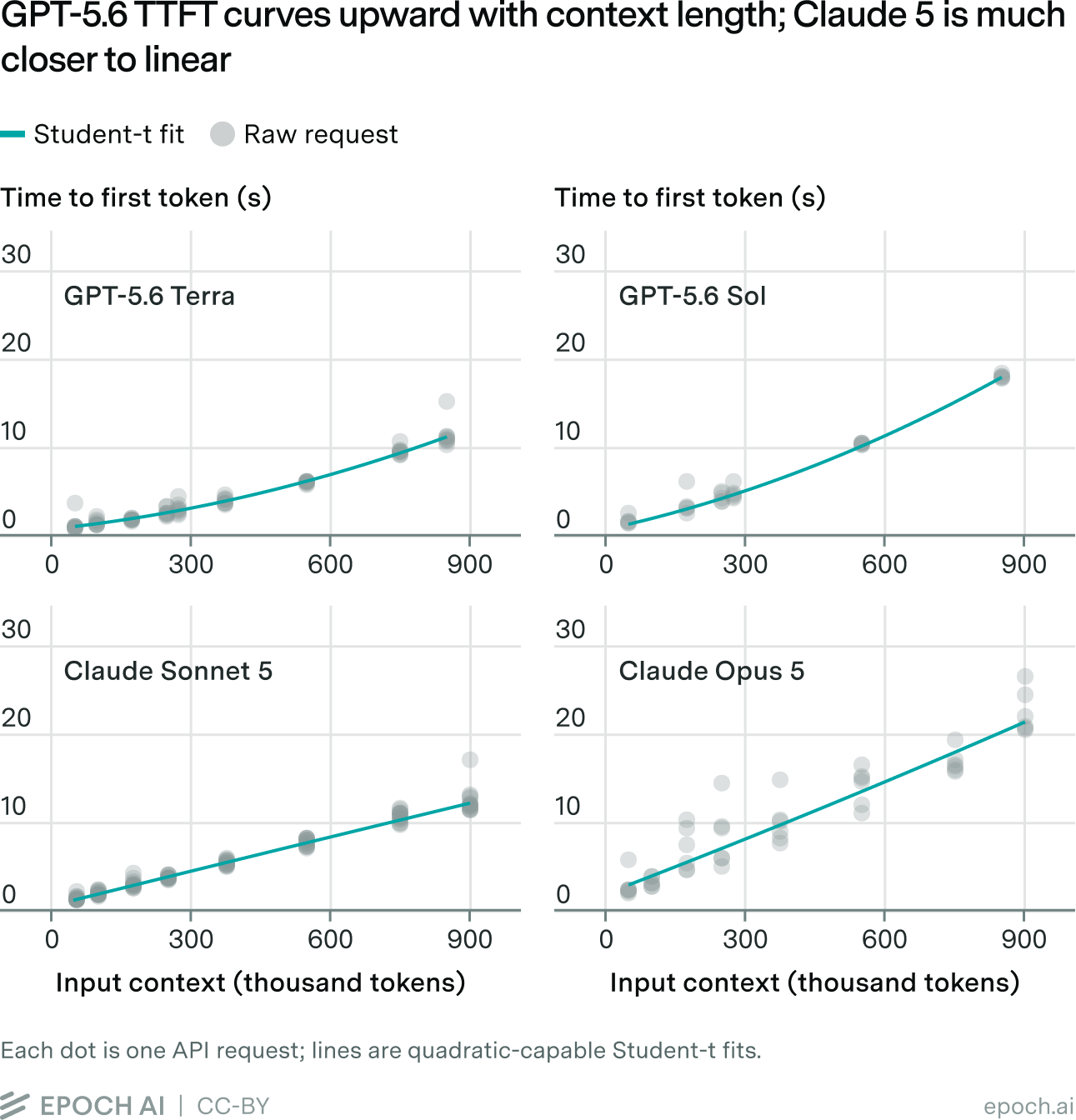
We measured how the time to first token (TTFT) scales with context length for OpenAI’s GPT-5.6 Terra and Sol and Anthropic’s Claude Sonnet 5 and Opus 5. We found that the two model families behaved very differently. Terra and Sol showed clear upward curvature as prompts got longer, consistent with a significant quadratic component. Sonnet 5 stayed close to linear scaling with no observable curvature, while Opus was noisier but still consistent with linear scaling. To test for the effect of noise in measurements, we fitted three estimators with different assumptions about the latency noise, and found that all three recovered similar curvatures for GPT-5.6 while keeping the Claude fits much closer to linear.
This result suggests that OpenAI and Anthropic have made very different architectural choices in how their respective models process long-context prompts. Claude’s near-linear scaling suggests that full attention, where each token attends across the entire context length and compute scales quadratically with context length, contributes much less to long-context processing than it does for GPT.
GPT and Claude show different long-context latency scaling
We measured TTFT with reasoning disabled across context lengths for four models: GPT-5.6 Terra, GPT-5.6 Sol, Claude Sonnet 5, and Claude Opus 5. Details of the measurement setup are provided in the appendix.
We fit a quadratic curve to each model using the Student-t estimator. Analysis of all four datasets uses the same quadratic specification:
\[\mu(x) = \alpha + \beta x + \gamma x^{2}\]Terra and Sol show a noticeable curvature. Sonnet is visually linear. Opus has noisier data than Sonnet but is similarly close to linear. In other words, for GPT-5.6, adding the same number of tokens leads to progressively larger increases in TTFT as the context grows, whereas for Claude, the added latency remains much closer to constant.
The difference is robust to different treatments of API latency noise
TTFT benchmarks can be noisy. We designed our experiments to minimize this, but there is clearly still significant noise in our results, especially for Opus. Some TTFT variation likely stems from the model execution itself, but our working hypothesis is that much of it arises from higher-level serving delays, such as queueing and routing. This motivates our use of estimators that treat a substantial part of the latency noise as positive additive delay rather than symmetric measurement error.
To test robustness to this noise, we repeat the analysis using two new estimators that treat latency noise differently: stochastic-frontier regression and a spike-plus-contention model. Both explicitly model additional positive latency from contention, while Student-t regression reduces the influence of extreme observations. Because the estimators target somewhat different notions of underlying latency, their fitted levels need not agree; the relevant test here is whether they agree on the shape of the relationship with context length. Full model specifications are given in the appendix.
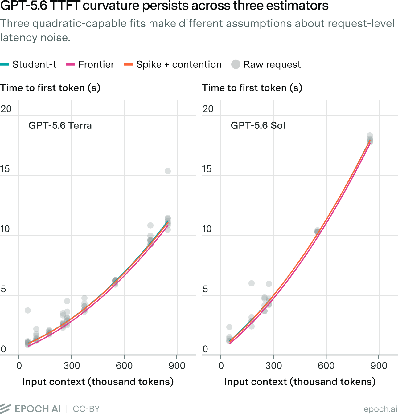
As expected, the estimators fit slightly different curves, but all three still agree on the curvature. Therefore, we can say that the quadratic scaling behavior is unlikely to be due to outliers pulling the curve upward.
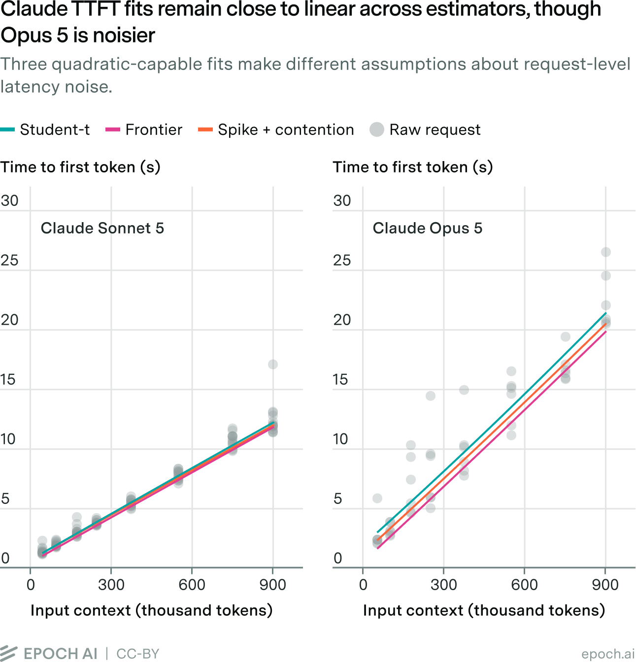
Sonnet has the cleanest results. The data show that the fit is very close to linear across all three estimators. Opus is much noisier, but the three estimators still produce fits with minimal curvature. Figures 1–3 together show that the tested GPT and Claude models have clearly different scaling curves.
Long-context efficiency has become a design choice
Traditionally, transformer-based LLMs have used full-attention layers, where each token attends to all preceding tokens. Therefore, the total attention compute to process a prompt scales quadratically with prompt length. Many open model families have moved toward more efficient long-context scaling. Hybrid models such as Kimi K3 and Qwen3.5 mix linear attention layers with a much smaller number of full-attention layers, specifically a 3:1 ratio. This decreases the number of full-attention layers by a factor of four, and therefore the quadratic term by the same factor. Qwen3.8-Flash-Next and GLM-5.3-Flash have moved further in this direction by replacing the full-attention layers with sparse attention. Sparse attention layers have a smaller quadratic component compared to full attention while still being able to attend to the entire context length. Sliding-window attention is another well-known technique; it was present in OpenAI’s open-source gpt-oss models. With a fixed window size, sliding-window attention has roughly constant attention cost per token and a linear total cost with sequence length. The common direction across all of these models is to reduce the amount of quadratic computation required at long contexts.
Our results suggest that Anthropic has also approached latency scaling in this way, at least for the models we evaluated. Sonnet and Opus both appear to have much smaller quadratic curvature than the GPT models. This is also in line with the fact that all Claude 5 generation models in Claude Code support a 1-million-token context window by default. In contrast, OpenAI appears to be making a different tradeoff. Although the GPT-5.6 family of models supports a 1.05-million-token context window, Codex defaults to autocompacting before 272,000 tokens. OpenAI has described avoiding context bloat as a key design goal for Codex. High-ranking OpenAI employees have publicly stated that they do not recommend increasing Codex’s default 272,000-token context window, despite official support for up to 1.05 million.
Cost implications of different architectures
Here is an illustrative example using Anthropic’s API pricing for Opus 5 for a 100,000-token request:
| Component | Calculation | Cost |
|---|---|---|
| Cached Input | 100k tokens × $0.50 / Mtok | $0.05 |
| Input (5-min cache write) | 1k tokens × $6.25 / Mtok | $0.00625 |
| Output | 1k tokens × $25.00 / Mtok | $0.025 |
| Total | $0.08125 |
Table 1. Hypothetical API cost for an Opus 5 request with 100,000 tokens of cached context, 1,000 new input tokens, and 1,000 output tokens.
If instead the context were 900,000, the cached input alone would cost $0.45. If cached-input pricing doubled, as with the GPT-5.6 models, the cached-input cost would rise 18× rather than 9× when increasing from 100,000 to 900,000 tokens of context.
So while Claude pricing stays constant, the increase in context results in a significant increase in cost. In contrast, Codex defaults to autocompacting before the 272,000-token threshold, which keeps contexts bounded in size and costs lower. It is possible that OpenAI is betting that 1-million-token contexts are often unnecessary, or that the cost savings offset any performance loss from shorter contexts.
Extrapolating to multi-million-token contexts
Within the supported context window of up to approximately 1 million tokens, the difference is not large enough to make GPT uneconomical. A doubling in price may still be acceptable for many long-context use cases. However, we can also consider how this might change if both model families hypothetically had longer context windows.
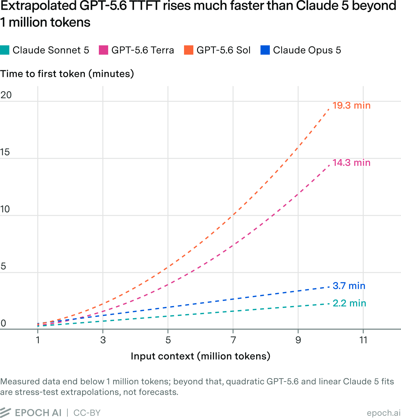
To illustrate this, we extrapolate the fitted scaling relationships to contexts of up to 10 million tokens. We used the existing quadratic fits for the GPT models and linear fits for the Claude models. To be clear, we do not claim that the Claude models are completely linear in scaling, but rather that the quadratic coefficient is small enough to approximate with a linear fit. We treat this as a stress test rather than a latency forecast. The measurements themselves extend only to roughly one million tokens, and models or serving systems could behave differently outside that range.
Another way to see the divergence is to look at the marginal TTFT cost of adding another 10,000 tokens at different context lengths.
| Model | At 0.1M context | At 1M context | At 10M context |
|---|---|---|---|
| GPT-5.6 Terra | 0.071 s | 0.216 s | 1.66 s |
| GPT-5.6 Sol | 0.136 s | 0.324 s | 2.20 s |
| Claude Sonnet 5 | 0.129 s | 0.129 s | 0.129 s |
| Claude Opus 5 | 0.218 s | 0.218 s | 0.218 s |
Table 2. Marginal TTFT added by an additional 10,000 input tokens at different context lengths. The 10M values are extrapolated beyond the measured range. Claude models use a linear extrapolation, so the marginal time is constant.
Extrapolating to these higher contexts makes the significance of the scaling difference clearer. At 10 million tokens, the quadratic curves for the GPT models imply roughly a 7–8× increase in marginal TTFT per additional token relative to 1 million tokens. This would greatly decrease the feasibility of serving these models.
This creates a different tradeoff for long-horizon agentic systems. If serving costs continue to scale linearly with context at these higher token limits, it could become economical to keep more history in the agent’s context as memory. This would allow the memory to be handled at the model level. If serving costs instead scale quadratically with context, then it may be better to use external memory systems and aggressive compaction.
Appendices
Appendix A: Measurement setup
A.1 Request construction and shared-prefix caching
For each model, prompts were crafted as follows.
{fixed cached prefix}{16-digit nonce}{target-length-specific text}{fixed task instruction}The 16-digit nonce is a unique number which changes for each request. The target-length-specific text is a chunk of text from the combined Project Gutenberg text. The breakpoint is placed before the nonce so that the nonce serves as the exact cache breakpoint. The changing nonce ensures that no prefix cache hit is possible past it. The task instruction was fixed: “Do not think or analyze. Respond immediately with exactly one word: OK”. For requests to the same model at a fixed context length, only the nonce part of the prompt changes.
OpenAI requests used an explicit prompt-cache breakpoint, explicit cache mode, and one session-specific prompt_cache_key. Anthropic requests used an explicit cache breakpoint with a five-minute TTL. Prompts for the GPT models were identical (except for the nonce changing per request). The same applies for the Claude models. This is because the tested models had the same token counts for our prompts within each family.
We targeted a size of 2048 for the cached prefix. The realized size was 2051 for the GPT models, and 2052 for the Claude models. The remaining text ranged from about 48,000 to 898,000 tokens. A cache warmup request was first sent with just the stable prefix and an uncached nonce. We confirmed that every measured request reported exactly the expected number of cached tokens (2051 and 2052 for GPT and Claude models respectively).
Our regressions used the nominal context length which was calculated beforehand using a placeholder nonce and slightly different ending. The actual provider-reported input lengths were exactly 2 tokens short for OpenAI, and 6 tokens short for Anthropic when compared to nominal.
A.2 Why TTFT is informative at long context
Inference is separated into distinct phases of prefill and decode. Prefill is the processing of input tokens, while decode is the processing of output tokens. Input tokens can be processed in parallel during prefill, while decode tokens must be generated autoregressively one at a time. At sufficiently long contexts, this can make prefill compute-bound once there are enough input tokens to saturate the available compute resources. TTFT includes prefill, generation of the first output token, and other serving and network overheads. At long context lengths, prefill can take many seconds, meaning that prefill time should make up a larger fraction of measured TTFT. We therefore expect TTFT to be informative about the time required for prefill and how it scales with context length, while recognizing that it also includes serving-system overheads.
A.3 TTFT timing and request execution
Requests were sent sequentially. Each model used one persistent HTTP connection. We waited for each request to finish before sending the next. Reasoning and thinking were disabled, and the responses were confirmed not to use reasoning tokens.
TTFT was measured with a monotonic clock from immediately before sending the HTTP request to the first nonempty streamed text delta. Prompt assembly, token counting, serialization, and request construction occurred before the timer started; measured TTFT includes request upload, network time, routing and queueing, cache lookup, prefill, first-token generation, and the return path.
A.4 Randomized chronological blocks
Requests were sent in blocks, with one request at every tested context length in each block. The loop targeted four seconds between request dispatches. Median recorded request-start intervals were 4.01 seconds for Terra, 4.75 for Sol, 4.39 for Sonnet, and 9.00 for Opus. Longer requests pushed the interval above four seconds.
Table A1.
| Model | Context lengths tested | Repetitions | Total requests |
|---|---|---|---|
| Terra | 50k, 100k, 175k, 250k, 275k, 375k, 550k, 750k, 850k | 8 | 72 |
| Sol | 50k, 175k, 250k, 275k, 550k, 850k | 5 | 30 |
| Sonnet | 50k, 100k, 175k, 250k, 375k, 550k, 750k, 900k | 14 | 112 |
| Opus | 50k, 100k, 175k, 250k, 375k, 550k, 750k, 900k | 6 | 48 |
We shuffled context order within each block to interleave short and long prompts over time and reduce confounding between context length and changing serving conditions.
Each regression also includes a sum-to-zero fixed effect for each block to account for changes in baseline latency between blocks, such as changing network or serving conditions. Dropping the block effects leaves the Terra, Sol, and Sonnet curvature estimates nearly unchanged. The Opus point estimate is more sensitive to the block specification, but the linear-versus-quadratic conclusion is unchanged.
A.5 Why use a shared prefix?
We adopted the shared-prefix method after early Claude runs with caching disabled showed very high TTFT variability at each context length. After adopting the shared prefix, we found that the variability decreased substantially. For Sonnet 5 specifically, median absolute deviation dropped from 0.318 to 0.136 seconds at 100,000 context and from 0.352 to 0.107 seconds at 250,000 context. Despite this improvement, Opus still remained significantly noisier than other models.
We did not do in-depth studies comparing cached versus uncached. The purpose of the shared prefix is to hold cache identity fixed. We hypothesize that the reduced noise may reflect a narrower serving cohort or more stable routing. For example, cache affinity might mean that all requests route to the same datacenter or worker engine. While there is some documentation on how routing may change based on cache, there is not enough information for us to make any concrete statements about it.
Appendix B: Common scaling model
For request \(i\) in block \(j\), \(y_{ij}\) is the observed TTFT and \(x_i\) is the input length in millions of tokens. We fit
\[\mu_{ij} = \alpha + \beta x_i + \gamma x_i^{2} + \delta_j\]where \(\mu_{ij}\) is the fitted latency and \(\delta_j\) is a block effect, with
\[\sum \delta_j = 0\]The linear fit sets \(\gamma\) = 0.
We use the same latency curve for all three estimators below. What changes is how the remaining variation in TTFT is treated.
Appendix C: Student-t regression
Our main fit uses a Student-t likelihood with four degrees of freedom:
\[y_{ij} \sim t_4(\mu_{ij}, \sigma)\]The heavy-tailed likelihood limits the influence of unusually slow requests. We leave \(\gamma\) unconstrained, so the fitted curve is free to have positive, zero, or negative curvature.
Appendix D: Stochastic-frontier regression
As a robustness check, we also fit a model where some of the measured latency can come from additional positive delay:
\[y_{ij} = \mu_{ij} + \epsilon_{ij} + d_{ij}\]\[\epsilon_{ij} \sim N(0, \sigma^{2})\]\[d_{ij} \sim \mathrm{Exponential}(\lambda), \quad d_{ij} \geq 0\]Here \(\epsilon_{ij}\) is the symmetric residual term. The \(d_{ij}\) term represents extra latency that can only increase TTFT, for example from queueing or other serving contention.
For this fit we constrain \(\beta\) ≥ 0 and \(\gamma\) ≥ 0. The resulting \(\mu_{ij}\) curve can be interpreted as an estimate of latency with the modeled positive delay removed.
Because the exponential term is continuous, every request receives some positive modeled delay, even if that delay is very small.
Appendix E: Spike-plus-contention regression
The frontier model does not allow a request to have exactly zero contention delay. We therefore also fit a mixture model that does:
\[y_{ij} = \mu_{ij} + \epsilon_{ij} + C_{ij} d_{ij}\]\[\epsilon_{ij} \sim N(0, \sigma^{2})\]\[C_{ij} \sim \mathrm{Bernoulli}(\pi)\]\[d_{ij} \sim \mathrm{Exponential}(\lambda)\]If \(C_{ij}\) = 0, the request has no modeled contention delay. If \(C_{ij}\) = 1, it receives an additional positive delay drawn from the exponential distribution.
The fitted \(\pi\) is therefore the estimated mixture probability for the contended component, while \(1/\lambda\) is the mean added delay conditional on contention.
As with the frontier fit, we constrain \(\beta\) ≥ 0 and \(\gamma\) ≥ 0. To prevent the clean-component width from collapsing toward zero, \(\sigma\) is anchored using negative residuals from a quadratic Huber pilot fit and held fixed during each frontier and spike fit. The reported Huber intervals use a 5,000-replicate whole-block bootstrap of a quadratic Huber refit, while frontier and spike-plus-contention intervals use 200 whole-block bootstrap replicates with \(\sigma\) re-estimated in each replicate. Requests from the same chronological block are resampled together.
Appendix F: Final fit results
Table A2. Student-t quadratic fits, with x measured in millions of input tokens:
| Model | α | β | γ | σ |
|---|---|---|---|---|
| Terra | 0.6509 | 5.5426 | 8.0265 | 0.2329 |
| Sol | 0.5939 | 11.5657 | 10.4159 | 0.2828 |
| Sonnet | 0.4665 | 13.1185 | -0.2058 | 0.3039 |
| Opus | 1.7975 | 20.3596 | 1.5754 | 1.4844 |
Table A3. Student-t linear fits, with x measured in millions of input tokens:
| Model | α | β | σ |
|---|---|---|---|
| Terra | -0.2774 | 12.6392 | 0.5100 |
| Sol | -0.7775 | 21.2691 | 0.6930 |
| Sonnet | 0.4890 | 12.9376 | 0.3044 |
| Opus | 1.6023 | 21.7917 | 1.4935 |
Table A4. Student-t block-effect sensitivity:
| Model | γ without blocks | γ with blocks |
|---|---|---|
| Terra | 7.7728 | 8.0265 |
| Sol | 10.4687 | 10.4159 |
| Sonnet | -0.1932 | -0.2058 |
| Opus | -0.2177 | 1.5754 |
Table A5. Quadratic-versus-linear evidence:
ΔAICc is defined as AICc_linear − AICc_quadratic, so positive values favor the quadratic model.
| Model | 2Δlog L | LR p | ΔAICc | Huber 95% γ interval | Huber % γ > 0 |
|---|---|---|---|---|---|
| Terra | 78.30 | 8.87 × 10⁻¹⁹ | 75.50 | [6.82, 9.12] | 100% |
| Sol | 41.05 | 1.48 × 10⁻¹⁰ | 37.29 | [8.97, 13.04] | 100% |
| Sonnet | 0.138 | 0.711 | -2.65 | [-1.22, 1.29] | 51.3% |
| Opus | 0.147 | 0.701 | -2.90 | [-6.30, 9.70] | 55.5% |
Table A6. Whole-block bootstrap γ intervals for the asymmetric estimators:
| Model | Frontier 95% γ interval | Spike 95% γ interval |
|---|---|---|
| Terra | [6.65, 8.55] | [6.27, 8.85] |
| Sol | [9.34, 12.64] | [9.31, 11.03] |
| Sonnet | [0, 0.93] | [0, 1.03] |
| Opus | [0, 8.33] | [0, 8.24] |
The results strongly support positive curvature for Terra and Sol. Sonnet is at the zero-curvature boundary in both asymmetric point estimates, while Opus remains inconclusive.
Appendix G: GPT-6 Astra
Measurements of Astra’s TTFT scaling show that it still has a significant quadratic component, similar to the GPT-5.6 models.
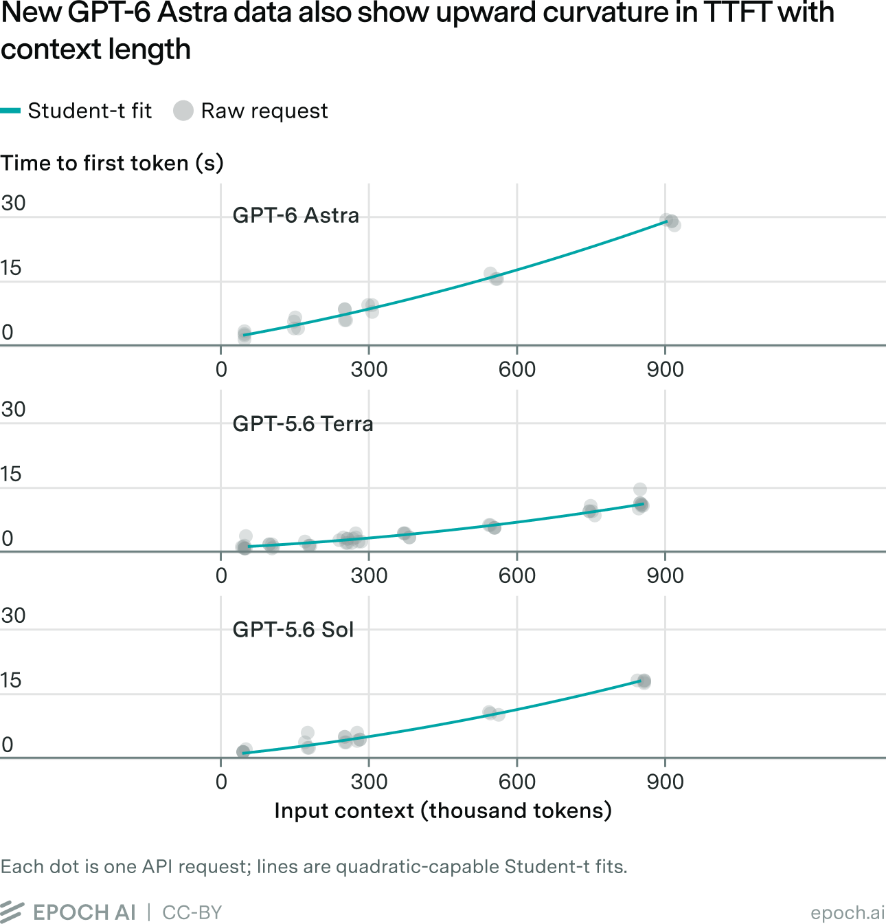
Table A7. Quadratic-versus-linear evidence for GPT-6 Astra:
| Model | 2Δlog L | LR p | ΔAICc | Huber 95% γ interval | Huber % γ > 0 |
|---|---|---|---|---|---|
| GPT-6 Astra | 26.73 | 2.34 × 10⁻⁷ | 22.67 | [8.62, 16.24] | 100% |
Table A8. Student-t quadratic fits for GPT-6 Astra, with x measured in millions of input tokens:
| Model | α | β | γ | σ |
|---|---|---|---|---|
| GPT-6 Astra | 1.4814 | 20.4760 | 11.6319 | 0.4858 |
Appendix H: GPT-6 Sol and GPT-6.1 Sol
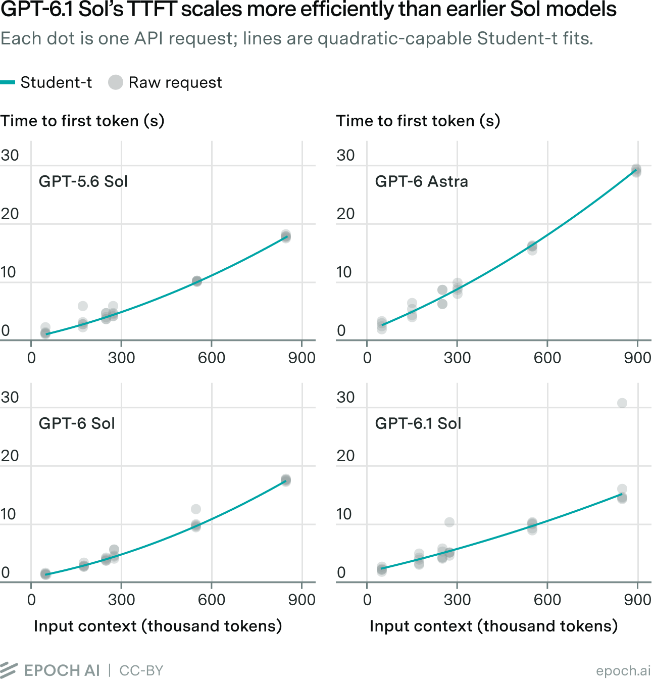
We extended our measurements to GPT-6 Sol and GPT-6.1 Sol. GPT-6 Sol closely follows GPT-5.6 Sol across the measured context range. GPT-6.1 Sol is slower at the shortest context tested, but its latency grows more slowly and is lower at the longest context.
| Fitted quantity | GPT-6 Sol | GPT-6.1 Sol | 6.1 versus 6 |
|---|---|---|---|
| TTFT at ~50k tokens | 1.32 s | 2.34 s | 1.02 s higher (77%) |
| TTFT at ~850k tokens | 17.43 s | 15.14 s | 2.29 s lower (13%) |
| Quadratic coefficient γ | 11.70 | 4.77 | 59% lower |
For the fitted baseline \(\mathrm{TTFT} = \alpha + \beta x + \gamma x^{2}\), TTFT is in seconds and \(x\) is in millions of input tokens. Values are fitted point estimates.
Appendix I: Code
Code for the benchmark, model fitting, and reproduction of the figures is available in the repository: