

Introduction
We investigated progress trends on four capability metrics to determine whether AI capabilities have recently accelerated. We do this by fitting several candidate curves to historical data (for example, a simple linear trend vs. a hyperbolic trend) and comparing how well each curve predicts data it hasn’t seen yet.
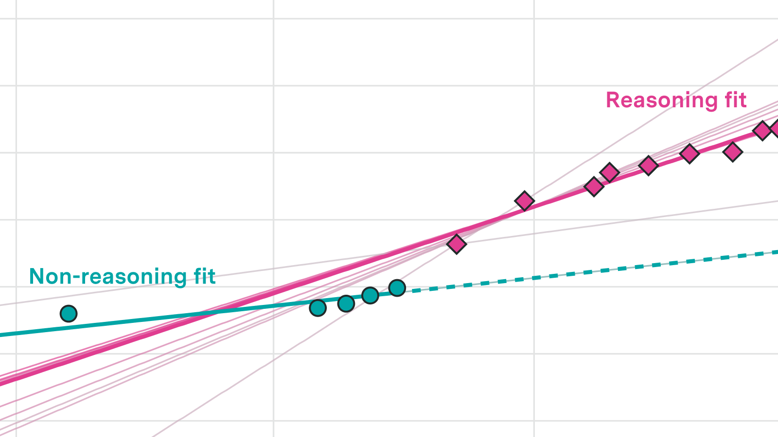
The following interactive plot shows how each candidate curve fits the historical data. Use the tabs to switch between the time series view and the cross-validation accuracy of each curve.
Three of four metrics show acceleration, seemingly driven by reasoning models
Three of the four metrics (ECI, log METR 50% time horizon, and a math-focused index we constructed from several math benchmarks) show strong evidence that progress has sped up relative to a global linear trend fit to data from 2023 onward.
The best-performing model across these three metrics was a pair of independent linear trends: one for reasoning models and one for non-reasoning models. Reasoning models show both a one-off jump in performance and a roughly 2-3x faster trend compared to non-reasoning models. That said, for any individual metric several other superlinear fits also perform well, so we cannot pin down a precise growth rate.

We have been calling this the “reasoning” / “non-reasoning” split, but this is not a perfectly clean dichotomy. Several correlated but not strictly identical changes happened over the same few months: scaling inference compute, heavier use of RL in post-training, and models producing reasoning tokens. Around that time is when we see an acceleration in capabilities.
Our fourth metric, an index constructed from WeirdML V2 results, showed no sign of acceleration. A single global linear trend fit the data best. One possible explanation is that WeirdML V2 places models in an unusually resource-constrained environment: models get only five attempts to submit working code, with no access to external tools. This setup has not been the focus of recent RL training, which may explain why progress there has not accelerated in the way we see on other metrics. However, we also have only about one year of pre-reasoning-model data for WeirdML V2, so there is limited statistical power to detect a break.
A note on generalizability. The three metrics where we find acceleration are concentrated in programming and mathematics. These are areas that labs have explicitly targeted for improvement, and they share an important property: correctness is easy to verify automatically, making them natural targets for reinforcement learning. Tasks where correctness is harder to verify may not have seen the same speedup, so the acceleration we document here may not be as general as the headline numbers suggest.
In conclusion, we show there has been a clear acceleration in several AI metrics of interest, seemingly corresponding with the release of reasoning models in 2024. The limiting factor for this analysis are benchmarks which can span a sufficiently large range of LLM releases, but we would be interested in including additional benchmarks in future, especially those covering domains outside of programming and mathematics.
Methodology
AI Capability Metrics
We use four AI capability metrics:
ECI (Epoch Capabilities Index), accessed from the “epoch_capabilities_index” within Epoch’s benchmark data archive. We augment this with a GPT-3.5 result previously calculated for an earlier Epoch trend analysis, extending the dataset back to March 2022.
METR 50% Time Horizon (version 1.1), accessed from METR’s published benchmark results. We work with the natural logarithm of the time horizon, which puts it on an approximately linear scale. We log-transform Time Horizon values to put progress on an approximately linear scale.
Combined Math Index. We construct a composite math benchmark from per-question results on MATH Level 5, Frontier Math 1-3 and 4, and OTIS Mock AIME 2024-2025 (sourced from Epoch), supplemented with results from MathArena. Because these benchmarks vary in difficulty and scoring, we need a principled way to place all models on a common scale. We do this using a two-parameter logistic (2PL) item response theory model, which estimates a latent “ability” parameter for each model while accounting for differences in question difficulty and discrimination across benchmarks.
In our 2PL item response theory model, each model’s predicted probability of answering question \(j\) correctly is \(\sigma(a_j (\theta_i - b_j))\), where \(\theta_i\) is the model’s ability, \(a_j\) is the question’s discrimination, and \(b_j\) is its difficulty. We select the median-difficulty question from the set with maximum model coverage and standardize it to \(a=1, b=0\). Parameters are estimated by minimizing binary cross-entropy with ridge penalties (\(\lambda_a = 0.378\), \(\lambda_b = 0.0001\)), chosen so that 95% of item slopes fall within a factor of 10 of the median. The resulting ability scores are linearly rescaled so that Sonnet 3.5 maps to 130 and GPT-5 maps to 150, for comparability with ECI.
WeirdML V2 Index. We construct a similar index from per-attempt, per-question classification accuracy results from WeirdML V2.
The IRT model here is adapted to account for WeirdML V2’s non-trivial guessing floor and performance ceilings on some questions. We first transform raw accuracy as \(p_{\text{transformed}} = \max(0, (p_{\text{raw}} - \text{guessing}) / (\text{max} - \text{guessing}))\), using benchmark-provided values for guessing rates and ceilings. We then fit the same 2PL model but minimize squared prediction error rather than binary cross-entropy (since the transformed values are continuous).
Dataset preparation modes
For each AI capability metric, we prepare the data in four ways to check robustness:
SOTA on release: each data point is a model that achieved strictly higher performance than all previous releases (the default approach used by Epoch and METR in prior analyses).
Named releases: mainline numbered releases from OpenAI, Anthropic, and Google DeepMind, excluding minor variants.
Daily max: converts SOTA-on-release data to daily resolution by carrying forward the best available performance on each day.
Daily interpolated: like daily max, but linearly interpolates between consecutive SOTA releases rather than carrying forward a flat value. This avoids the issue where a higher cadence of releases mechanically looks like faster progress.
Our high-level conclusions are robust across these four modes.
Candidate fits
We fit eight parametric models to each dataset-mode combination, ordered from slowest to fastest implied growth:
- Global linear: \(y = a + bt\). Constant rate of progress.
- Reasoning split: two independent linear trends, one for reasoning models and one for non-reasoning, allowing both a level shift and a slope change when reasoning-capable models emerged.
- Piecewise linear: automatically selects either a global linear trend or a trend with a single breakpoint, chosen by BIC. (Implemented using the “segmented” R package with \(k = 0\) to 5 candidate breakpoints.)
- Log-augmented linear: \(y = a + t(b + c \cdot \ln(t))\). Growth that accelerates, but only logarithmically. (Constrained to \(c \geq 0\).)
- Quadratic: \(y = a + bt + ct^2\). Standard polynomial acceleration. (Constrained to \(c \geq 0\).)
- Power law: \(y = a + b(t + t_0)^p\), with \(p > 1\) and \(t_0 > 0\).
- Exponential: \(y = a + b \cdot e^{ct}\), with \(c > 0\). (Since METR time horizons are already log-transformed, this corresponds to double-exponential growth on the original scale.)
- Hyperbolic: \(y = a + b/(t_0 - t)\), with \(t_0 > 0\). Diverges at a finite time, representing a “singularity” model.
Time \(t\) is measured in years since the first observation in each dataset. Parameters are estimated by unweighted least squares.
Assessing fit quality
We compare fits using expanding-window cross-validation, which mirrors the forecasting use case. Starting from a minimum training set (chosen to give each curve at least 4-5 data points), we fit each model on the training window and evaluate predictions on all later data. The window then expands by one observation and the process repeats.
The minimum training cutoffs are: ECI (June 2024), METR Time Horizon (January 2024), Combined Math (September 2024), and WeirdML V2 (January 2025).
At each step we compute root mean square prediction error at five horizons: the next point only, and all points within 3, 6, 9, and 12 months of the training-set cutoff. We pre-selected the 6-month horizon as our primary metric, balancing genuine forecasting distance against the limited date range of our data.
For the SOTA-on-release and named-releases modes, we calculate errors in two ways: a “per-release” approach (averaging error over the model releases in each window) and a “daily-interpolated” approach (interpolating daily values between releases for evaluation, to prevent periods with more frequent releases from receiving higher weight). The daily-max and daily-interpolated modes are evaluated on their native daily values.
Constructing “best-performing fits” sets
To quantify uncertainty in model rankings, we use a leave-one-out stability analysis. For each combination of dataset, mode, and evaluation approach, we identify the best-performing curve (lowest mean RMSE at the 6-month horizon). We then test whether dropping any single observation (for per-release modes) or any contiguous 10% block of data points (for daily modes) would flip the ranking. A curve enters the “best-performing” set if it outperforms the overall best in at least 5% of these perturbations.
This is an approximate technique rather than a formal statistical test. It is meant to give a sense of which fits are “close to” the best, rather than to provide rigorous confidence intervals.