In their quest to make smarter AI, companies vie to build — and power — the largest datacenters.

xAI built the 350 MW Colossus datacenter in Memphis, which they plan to expand to 1.5 GW, while OpenAI’s 240 MW Abilene Stargate datacenter is planned to reach 1.2 GW. At full scale, these single datacenters will rival the most power-hungry facilities in the world today, such as the 1.2 GW Maaden or the 1.6 GW Bahrain aluminium smelters.

And if trends continue, companies might soon exceed this, with training clusters projected to reach 10 GW by the end of the decade. This is larger than the capacity of the US’s largest power plant, the Grand Colulee Dam, and nearly matches the total installed power capacity for all NVIDIA AI chips at the end of 2024.¹

But utilities are already struggling to supply the power AI hyperscalers demand. John Ketchum, CEO of the largest US utility, NextEra, stated last year that while some sites could readily support one gigawatt, it would “take some work” to accommodate 5 GW, let alone 10 GW. Mark Zuckerberg confirmed more recently on a podcast that energy constraints are bottlenecking AI, saying “we would probably build out bigger clusters than we currently can if we could get the energy to do it.”

There is a potential solution. Decentralized training could allow companies to build smaller datacenters in different grid regions – for instance, near existing power plants that each have a few hundred megawatts of spare capacity – and coordinate them as a single cluster to train frontier AI models.

Conventional wisdom in the field holds that large pretraining runs require large contiguous compute buildouts.

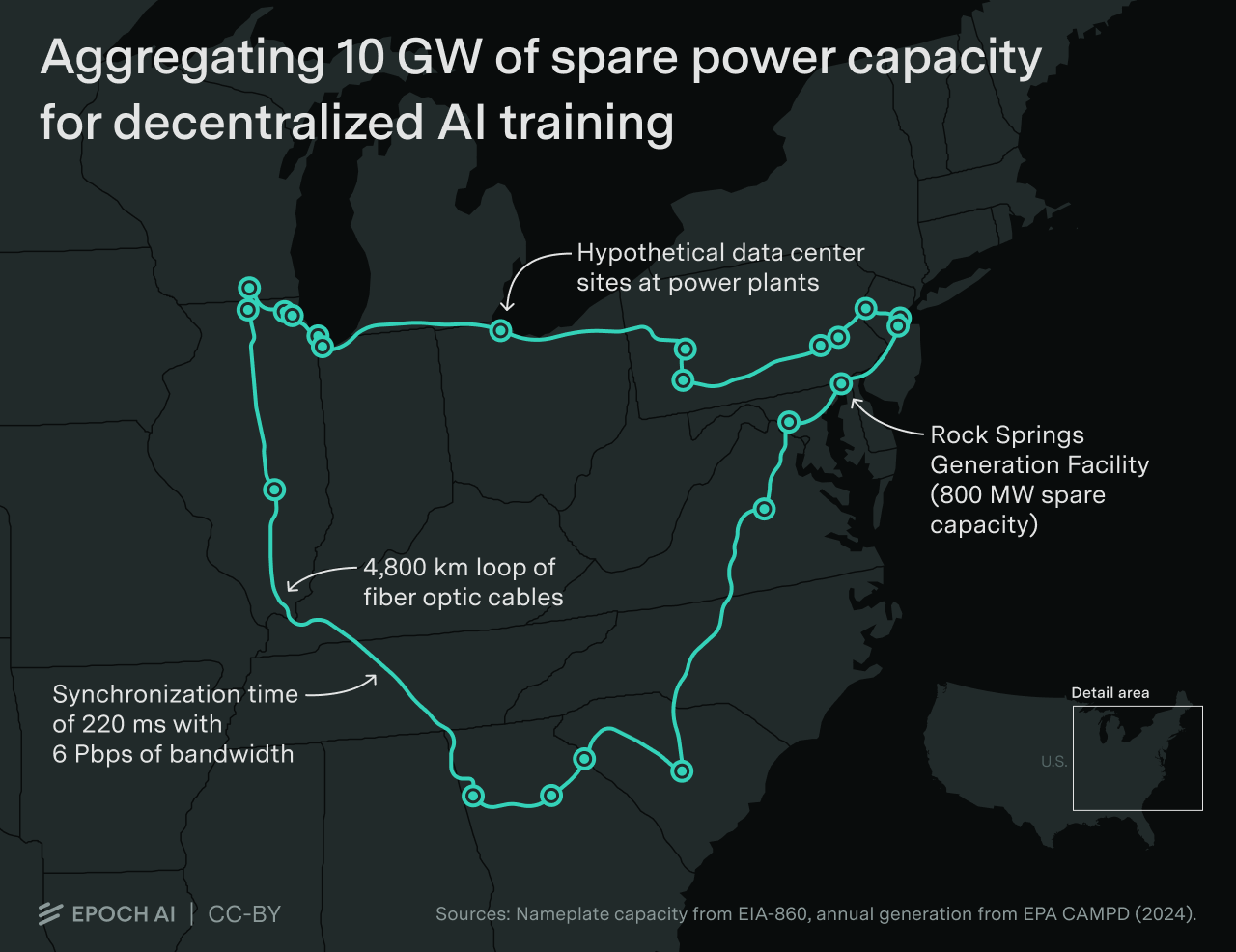
We believe this is wrong. In this article, we explore how decentralized training could be used to orchestrate a 10 GW training run, using spare capacity from 23 existing gas power plants, where nearby datacenters could be built and connected through a 4,800 km long fiber optic network. We explain how data parallelism could be used to coordinate such a run, the resulting latency and bandwidth requirements, and the cost of building the network relative to the datacenter sites. Finally, we analyze the pros and cons of conducting a 10 GW training run across multiple locations versus scaling a single campus.

We conclude that it is technically feasible to distribute training for multi-gigawatt-scale clusters across dozens of sites, thousands of kilometers apart, and have them coordinate on a large pretraining run. This would simplify the challenge of finding sufficient power in one location, without significantly increasing training times or construction costs, which may balance the additional engineering complexity decentralization would impose.

This suggests that while companies may prefer to minimize training constraints and permitting complexity by scaling giant campuses, AI scaling is unlikely to be deterred by utilities unable or unwilling to offer multi-gigawatt sites.

Planning a ten-gigawatt training run

First and foremost, we need to understand where power for datacenters could be available in the US today.

While there are few places that could handle a new 5 or 10 GW data center, there is existing under-utilized power generation infrastructure. The grid is built for peak load, but in many locations, peak loads are relatively rare. So grid utilization can be low, and there is more power available if we use the grid more efficiently.²

We compiled a list of gas power plants in the US with high spare capacity, as a proxy for overall power availability in the area (see the appendix for more details). The largest capacity-adjusted location we could find — the Rock Springs Generation Facility in Maryland — has approximately 800MW of spare capacity. This power plant is idle most of the year, producing only 2% of its nameplate capacity annually, only firing during peak loads for the local grid.

To scale the cluster to 10 GW, we will consider 23 existing power plants with spare capacity between 300 MW and 800 MW across the US East, spanning from Illinois to Philadelphia to Georgia. Hypothetically, data centers could be built at these sites and connected by 4,800 km of fiber optic cables to harness over 10 gigawatts of power.

In practice, it is unlikely that these specific powerplants will be ready to lend that much capacity to data centers, but it suggests that companies should be able to get that much power from nearby locations.

What kind of model would we train?

Ten gigawatts is a massive amount of power. It would support the installation of around 51,000 GB200 NVL72 servers (i.e. around 3.7M GPUs),³ capable of a collective throughput of 2e22 FLOP/s.⁴ Such a cluster would match the computational power of approximately all AI chips deployed today.⁵

This would be enough to conduct a 5e28 FLOP training run in about 100 days⁶ at at 30% model FLOP utilization (MFU)⁷ — a training run 100x larger than Grok 4, the largest training run to date.

What kind of model and training one would do with such a massive amount of compute is not clear. We will imagine pretraining a 72T parameter model with 4T active parameters per forward pass on 2,000T tokens.⁸ For comparison, the largest model we know the details of the training of — Llama 4 Behemoth — has 2T parameters, 288B active parameters, and was trained with over 30T tokens.

In practice, much of this compute would go instead towards synthetic data generation and RL rollouts instead of pretraining, which are easier to parallelise.⁹ We focus on a pure pre-training run as a worst-case stress test of the limits of decentralized training. We also focus on existing best practices and state-of-the-art hardware; a 10 GW cluster will likely use better hardware once it is eventually built.¹⁰

How would we decentralize training?

There are multiple ways to distribute a training run. We could split matrix multiplications across multiple nodes (tensor parallelism), distribute the computation of the different layers of a neural network (pipeline parallelism). But the most conceptually simple way to distribute training is at the level of data.

During each step of training, AI models process a large batch of data, which are used to determine the optimal direction in which to tweak the model parameters to improve performance, i.e. the gradients.

Instead of processing the whole batch in a single datacenter, we can split the computation across multiple datacenters, which would then synchronize before updating the model weights to aggregate the gradient — this is called data parallelism, and it is the same strategy Google used to split their training run of Gemini 2.5 across multiple, nearby datacenter buildings.¹¹ A similar strategy was tested in May by NVIDIA to train a 340B parameter model between two datacenters 1,000km apart.

Each batch will be split across datacenters in proportion to their computing capacity. Each site computes a local gradient during the computation phase, then exchanges their local gradients with each other. The aggregated result is used to update the copies of the model weights during the synchronization phase.

Within each datacenter, we will apply more data parallelism — as well as other types of parallelism such as pipeline and tensor parallelism — to split the computation of each local batch across all available machines. Coordinating this is already challenging, and requires careful engineering. For our purposes, we will consider that the intra-datacenter coordination challenges have already been solved. We will focus instead on the additional difficulty of coordinating data parallelism across distant sites.

Can decentralized training maintain sufficient throughput at very large scales?

From a technical standpoint, a decentralized training run will only make sense if the time spent communicating between data centers doesn’t slow down training too much.

Ideally, synchronization (i.e. the communication between datacenters) can occur partly in parallel with the processing, so it doesn’t slow down the training much. In the worst case scenario, with no overlap at all between synchronization and processing, the training would be slowed down by the time spent synchronizing.

We will aim for each synchronization to take no more than 5% as long as the time spent processing batches, so that at the worst it will increase total training time by 5% — or 5 days over what would be a 100 day training run in a centralized setup.

To analyze this, we need to know how long it takes to process each batch. Then, since we need to perform a synchronization per batch, we can check whether it’s possible to keep the communication time per synchronization under 5% of the batch processing time.

How long to process each batch?

The time it takes to process each batch is determined by the batch size and the total training time we aim for. Importantly, the batch size cannot be arbitrarily big — after it reaches a certain size we refer to as the critical batch size there are harsh diminishing returns to increasing its size.¹²

The best public work on determining the critical batch size we are aware of is from Bersgma et al. (2025), who posit that the critical batch size increases with roughly the square root of the training dataset size. Extrapolating their results suggests a critical batch size of 1.1B tokens for a 2,000T token training dataset. For reference, DeepSeek v3 was trained with a maximum batch size of 63M tokens.¹³

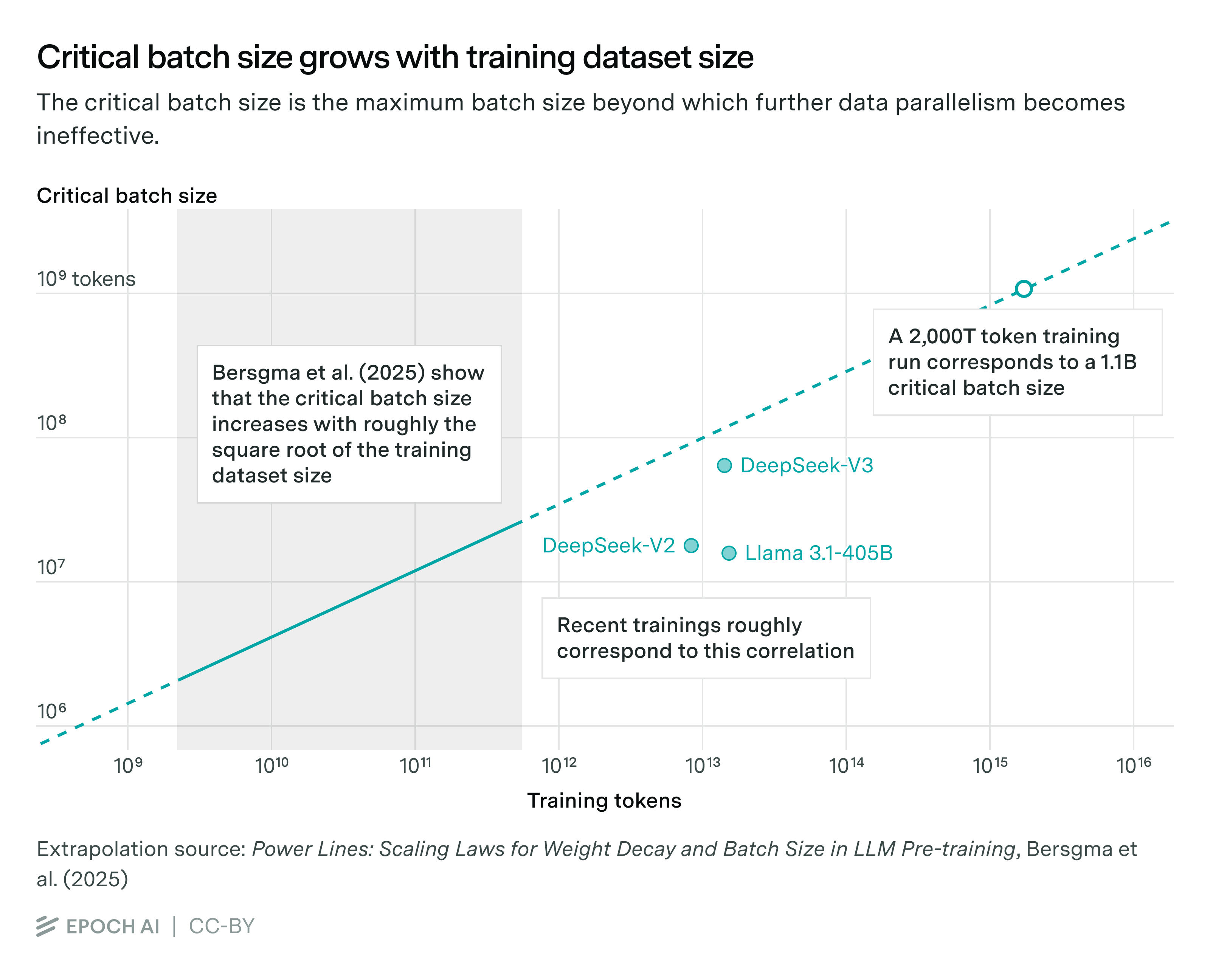
A 1.1B batch size makes for 2,000T training tokens / 1.1B batch size ≈ 1.8M gradient updates. If we want to finish training in under 100 days, then each batch should be processed in less than 100 days / 1.8M updates ≈ 4.8 seconds.

How much time will we spend on the network?

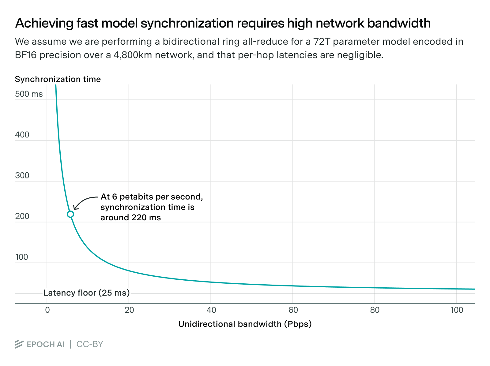
Based on a processing time of 5 seconds per batch, we will be aiming for a synchronization time of less than 250 ms – in order to guarantee that the decentralized training run will not be extended by more than 5% of the computation time, i.e. at most 5 more days of training on a 100 day training run.¹⁴

For synchronization between datacenters, we will use a bidirectional ring All-reduce algorithm. This allows for completing each synchronization in one round trip of the network, with an amount of communication between each pair of adjacent datacenters equal to the size of the model.¹⁵

The total time spent in the synchronization process is then determined by two factors;

• The propagation latency, which is determined by the network length and the propagation speed through fiber optic, plus the latency within the switches and networking hardware in each datacenter.
• The serialization delay, which is determined by the amount of data to be transmitted (determined by the model size), and the network bandwidth.

In our scenario, we would need to achieve a propagation latency and network bandwidth that would allow us to complete each synchronization step in under a quarter of a second.

Would the propagation latency be low enough?

If the data centres were merely connected over the internet, training would quickly become bottlenecked by communication. An enterprise internet connection of 10 Gbps and 100ms latency would only allow to transmit gradients for up to a 560M parameter model in under a second, nowhere near enough for the scale of modern AI training.¹⁶

However, AI datacenters will not communicate over the internet. Instead, companies lay down dedicated long-distance fiber optic connections between datacenters, explicitly reserved for training communications.

Long-distance communication latency is dominated by the length of the network and the propagation speed of fiber. Modern fiber optic can propagate signal at two-thirds the speed of light, for a latency of 5us/km.¹⁷ This would make our 4,800km network have a latency of 24ms.¹⁸

Each step in the network also contributes to the latency, requiring around 28us for the datacenter switches to convert the fiber optic signal to electric and back to an optic signal,¹⁹ and less than 1us per hop for communicating with the NVL72 servers.²⁰ Thus, the per-hop time adds negligible latency when distributing training across dozens of datacenters, though we would need to account for it if we intended to distribute across thousands of datacenters.

In sum, for a 4,800km long network with 23 sites, latencies are well below the target of 250 ms.

Could bandwidth be a bottleneck?

In order to transmit the gradients for our 72T parameter model, we would need a 6Pbps connection between each pair of adjacent datacenters in our network, in both directions. Accounting for latency, this would allow us to transmit the gradients in about 220ms²¹ – low enough to support synchronization in less than even 5% of the time it takes to process a batch.

This is a mind-boggling amount of bandwidth; for context, the MAREA transatlantic underwater cable has a system capacity of 200Tbps, 30 times lower than our hypothetical interdatacenter connection. However, as we will see in the next section, the costs of increasing network bandwidth are modest in comparison to the datacenter construction costs, making a 6Pbps connection quite affordable.

Learn more about our assumptions.

Parameters	Value	Notes
Number of datacenters	23	Number of sites across which we will do data parallel (DP) training.
Model size (T parameters)	72	Number of total parameters of the model. Recent large models have reached 1T parameters in size, while the Qwen team is supposedly planning training 10T parameter models.
Max network length (km)	4,800	Network length, corresponding to a ring joining datacenters nearby 23 gas power stations in the US east with over 100MW of spare capacity.
Fiber optic latency (s/km)	5.00E-06	White Paper on Huawei MS-OTN Low-Latency Network Solution, 5us/km, figure 2-2.
Per hop latency (us)	28.00	For example, the Cisco NCS 2000 400 Gbps XPonder Line Card Data Sheet lists a 28us end-to-end switch latency.
Transmission time (ms)	191	Flight time of the packages, excluding latency. We assume the gradients are communicated in BF16 format.

The total synchronization time is approximately given by

\[\begin{align*} \text{synchronization time} &= \underbrace{(\text{network length} \times \text{fiber latency}) + (\text{hop latency} \times \text{number of hops})}_{\text{network latency}} \\ &\quad + \underbrace{\frac{\text{model size} \times \text{bits per parameter}}{\text{network bandwidth}}}_{\text{serialization time}} \end{align*}\]

Would the NVL72 servers in each site be capable of supporting 6Pbps bandwidth in the first place? Each NVL72 rack is equipped with 18 compute trays, each with 4 ConnectX-7 400Gbps ethernet connection ports for external communication, for a total network bandwidth per NVL72 of 18 compute trays/NVL72 x 4 ports x 400 Gbps/port = 28.8 Tbps/NVL72. In our example network, the smallest node—corresponding to a site next to the NRG Rockford II power plant in Illinois—would have 300MW of installed capacity, enough to install ~1530 NVL72 GB200 servers, for a total ethernet bandwidth of 1530 NVL72 x 28.8 Tbps/NVL72 ≈ 44 Pbps. This bandwidth would be split between managing two links to the neighbouring datacenters in the ring and connecting separate buildings within each datacenter for intra-datacenter scaling. All in all, this should be enough to support two 6Pbps bidirectional connections per datacenter.²²

It would even be possible to reduce the synchronization time — while staying above the latency floor of 25ms — by further increasing the bandwidth. This would allow companies to use smaller batch sizes or reduce the training time overhead even more. For our article we will stick to a 6 Pbps connection, which will be enough to conduct the 10 GW training run we are considering.

Is the network cost feasible?

How expensive would it be to build such a network – a 4,800km, 6Pbps fiber optic network joining 23 datacenters? This cost breaks down into the installation of the fiber and the network equipment in the datacenters.

Typically, we would install the fiber underground, following along major highways. The cost of fiber underground installation is approximately $53,000/km. We would also need to pay for the cost of the fiber material, but this is much less expensive. With 800G per channel and 64 channels per pair, we would need about 120 fiber pairs to support a bidirectional 6Pbps point-to-point connection, which would cost around $6,700/km of fiber and casing material. The total installation cost of a 4,800 km fiber would then be roughly $290mn.²³

To make use of the fiber, the datacenters would need to be equipped with optic switches. The Broadcom’s Tomahawk 5 switch costs around $20,000 per unit,²⁴ and supports a 51.2 Tbps connection. We would then need 240 switches per datacenter to support a 6Pbps connection, which across 23 datacenters would cost in total $120mn.

In total, the cost of the network would be $410mn.

While expensive, the cost is small compared to the costs of datacenter construction: datacenter companies are offering to build datacenters at a price of about $12mn per megawatt of IT capacity, which for our 10 GW total capacity cluster would total $90bn.²⁵ This would make for less than a 1% increase in the price of the datacenter construction. This relative increase in price further dwarfs in comparison to the cost of the hardware equipment needed — the NVL72 racks alone would cost over 51,000 NVL72 x $3mn/server ≈ $150bn.

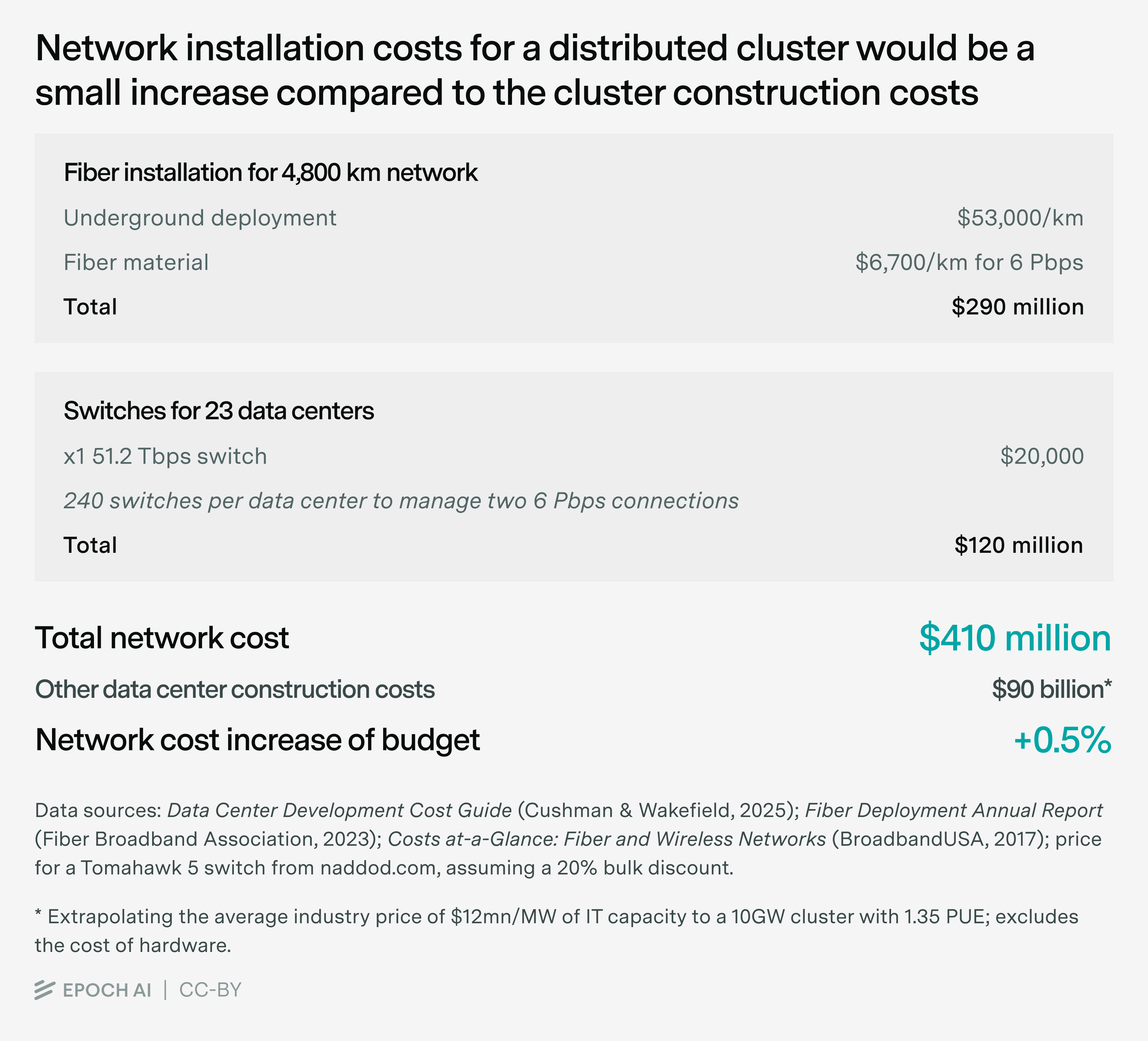
In sum, we conclude that a network 4,800km long with 6Pbps bandwidth could support a 10 GW decentralized training across 23 datacenters, incurring a potential delay of training of at most 5 days and an increase in datacenter construction costs of less than 1%.²⁶

Will companies actually turn to decentralized training at scale?

The bottom line is that it would be technically feasible to build a network with enough capacity to complete each synchronization step in a quarter of a second – making a 10 GW decentralized training run possible.

But will companies actually prefer them?

Large-scale decentralized training has many inherent disadvantages. Network links introduce additional points of failure, making any given training run less reliable than it would be on a single, locally networked cluster. Large-scale decentralized training adds engineering complexity, including more complex checkpointing, scheduling, and synchronization.

Actually building many geographically decentralized facilities and networking them together also presents its own challenges, including disparate permitting and regulatory regimes, and the local availability of skilled labor and materials. While the fiber costs would not be a large portion of the budget, arranging the necessary permits for interstate construction would be complex.

On top of this, centralized training is more future-proof. While any training scheme that works in a decentralized setup can be easily adapted to a centralized one, communication heavy protocols could only be supported by centralized clusters. While current trends in the AI field (towards e.g. more synthetic data generation and RL training) are decidedly friendly to decentralized setups, a new advance could upend this balance, giving an edge to centralized setups.

It is then not a surprise that AI companies today are planning large centralized AI clusters. For example, Crusoe claimed that their 1.8 GW Wyoming data center in collaboration with Tallgrass, currently under construction, is designed to scale up to 10 GW.

So when does it make sense to build large decentralized clusters?

Above all, decentralized setups open up more possibilities for building more cluster capacity. There are multiple reasons for this.

First, as in our example training run, it might be possible to leverage the spare capacity of existing power plants to build nearby (or co-located) datacenters. Norris et al (2025) find that 76 GW of existing spare capacity in the grid could be leveraged by new datacenters as long as they agree to throttle their GPUs during 22h per year to allow the grid to handle peak loads. This would favor a decentralized setup, with datacenters opportunistically located near available power.

Second, utilities are often reluctant to sign very large power purchase agreements, and make the accompanying capital investments in transmission infrastructure. They perceive a risk that AI energy demand could fall or new companies such as OpenAI could go bankrupt and default on their power purchase agreements – likely one reason why OpenAI and Anthropic have historically relied on larger tech partners to build datacenters for them, rather than borrowing to build their own datacenters. Because of this, utilities may prefer to contract for smaller loads in different grid regions, for which they could more easily find new customers if tenancy agreements fall through, and require less investment in grid infrastructure.

Third, the already lengthy grid interconnection requests take even longer for larger loads, with 200 MW+ interconnection requests taking over 55 months to be processed. Companies are bypassing interconnection queues to some extent by building off-grid power generation, e.g. the first stages of Meta’s Orion or XAI’s Colossus were supplied by hundreds of megawatts of off-grid power.

However, scaling off-grid generation up to gigawatts of power is no easy task, as it would require major infrastructure such as a large natural gas pipeline – to our knowledge, no AI datacenter planned today involves off-grid power generation over one gigawatt.

Generally, off-grid generation is considered a stopgap measure, with the eventual goal being on-grid energy. For example, Crusoe lists this as their explicit plan for Abilene, and xAI’s Colossus is already supplied by off-peak on-grid electricity (falling back to on-site generation during peak times). .

Fourth, larger loads create grid stability risks. A one gigawatt load is already substantial; a 10 gigawatt load exceeds the power consumption of entire US states. This problem is compounded by uncertainty of use — while loads during training are fairly predictable, later inference and research workloads fluctuate far more²⁷. This requires further investment in grid infrastructure, and potentially fine-grained resource coordination, with failures resulting in incidents like the infamous Spain blackout in April.

Finally, two lesser factors are worth noting.

Fifth, existing grid transmission lines aren’t usually rated for multiple gigawatts of power. Even the US’s highest capacity 765 kV two-circuit voltage corridors carry only 6-7 GW on their own over long distances. This limits the locations where grid-powered multi-gigawatt AI campuses can be built in the US without major new transmission infrastructure. We note however, that China, India, and the EU have installed high-capacity high-voltage DC transmission lines, with some cables carrying over 10GW, whereas the US is limited by geography and aging AC infrastructure.
Sixth, decentralized setups offer greater flexibility for future expansion. While large campuses are often planned in several successive stages to allow for subsequent expansions, decentralized networks can keep scaling beyond the original plan by linking additional datacenters.

These benefits might underlie Microsoft’s vision to build a decentralized Wide Area Network (WAN) of large AI datacenters “to enable large-scale distributed training across multiple, geographically diverse Azure regions”, with their Fairwater site in Wisconsin already planned to harness multiple gigawatts of power.²⁸

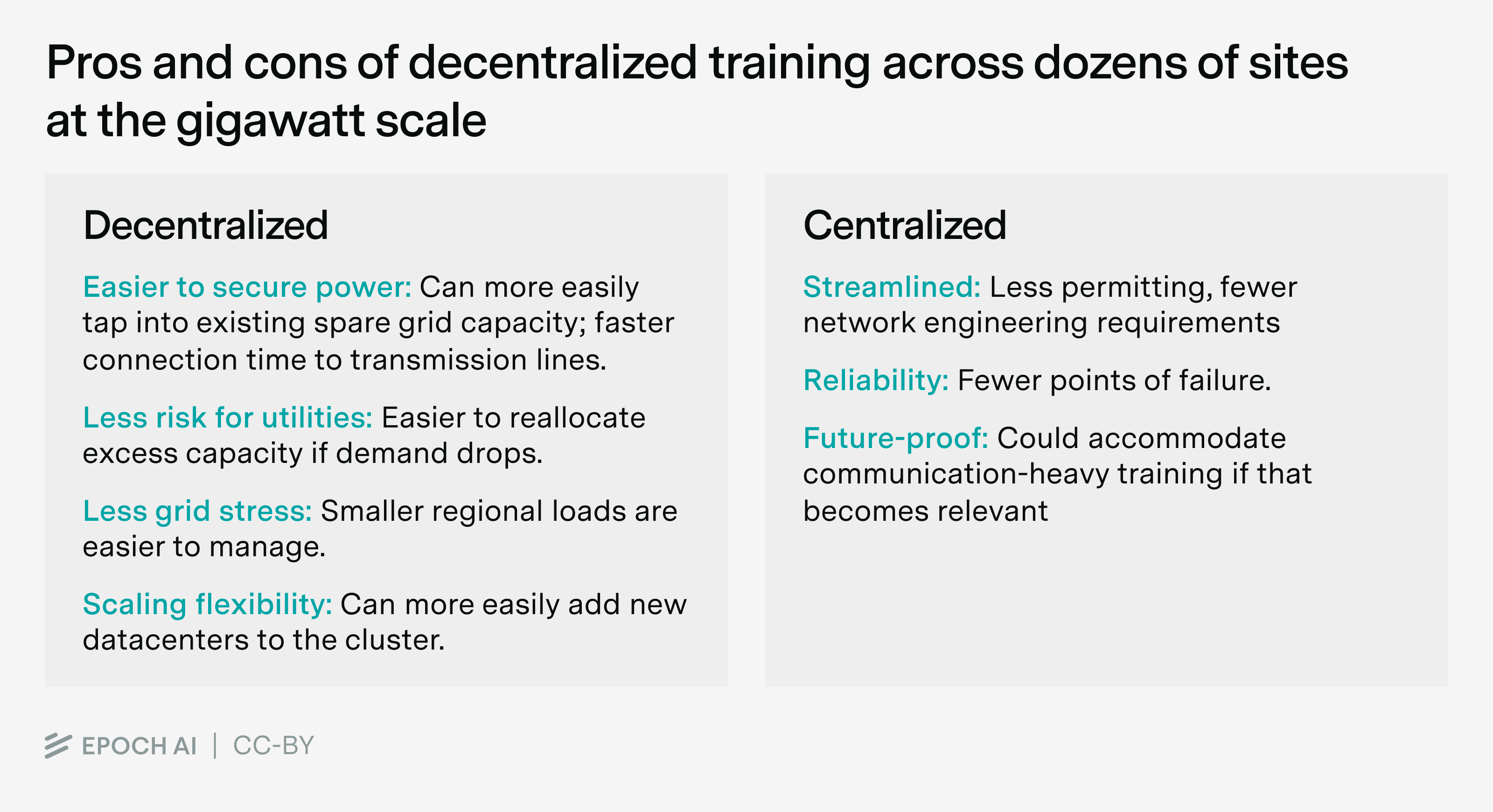
If the option exists, we expect companies would prefer single large campuses, to simplify training run complexity. However, decentralized clusters will make it easier to find suitable locations and coordinate with utilities, which favor smaller power plants across multiple regions to manage grid loads better.

We expect that companies will try to secure sites with as much power as possible, and only resort to decentralized clusters when no other option is available. In practice, we expect companies will build single sites ranging from megawatts to up to a gigawatt, while for scales over 10 GW they will prefer to build a decentralized cluster with individual locations ranging from hundreds of megawatts to a few gigawatts each.

Decentralizing training runs is easier than most think. Because of this, while securing power remains a major challenge, it is unlikely to significantly slow AI scaling.

---

We thank Jean-Stanislas Denain, Greg Burnham, Anson Ho, Daniel Ziegler, Ryan Greenblatt, David Schneider-Joseph, Ben Cottier, Arthur Douillard, Harqs Singh, Erich Grunewald, Sandra Malagón, Lennart Heim, Tim Fist, Yafah Edelman and Ron Bhattacharyay for their commentary and support.

Lynette Bye worked on editing and writing this report, Robert Sandler designed the article graphs.

Appendices

Appendix A: US power plant locations

Table of US gas power plants selected for our network.

A list of natural gas powerplants were found using the EIA form 860 (EIA-860) for 2024, sheet 3 (generators), aggregating across plant code, nameplate capacity > 300MW, and energy source (‘NG’).

Subsequently, annual generation data for each generator at each plant from EPA’s CAMPD from 2024 was used to compute a capacity factor / utilization fraction based on power generated VS nameplate power, which then gives the final capacity factor and estimate of available power.

More information is available in our companion spreadsheet.

Plant Name (EIA)	CF-adjusted Available Capacity (MW)	Lat.	Lon.
Rockspring Generating	779	39.71901	-76.15976
Troy Energy LLC	702	41.47724	-83.45983
Tenaska Virginia Generating	493	37.8667	-78.3813
LG&E Monroe	464	33.8148	-83.6954
Tenaska Westmoreland Generating Station	454	40.175247	-79.69667
Holland Energy Facility	447	39.223145	-88.75841
MPC Generating	382	33.8119	-83.6953
Sayreville Cogen	381	40.439	-74.3444
Columbia Energy Center	352	33.8697	-81.0178
Crete Energy Park	351	41.429443	-87.6187
AES Ironwood	350	40.3509	-76.3658
Hartwell Energy LP	343	34.33959	-82.81987
Calumet Energy Team LLC	312	41.6835	-87.5563
NRG Rockford II	307	42.23856	-89.1012
Armstrong Energy LLC	577	40.63802	-79.35173
MRP Elgin LLC	533	42.00006	-88.24457
Sewell Creek Energy	520	33.9486	-85.2769
Red Oak	514	40.448673	-74.34888
MRP Rocky Road LLC	414	42.0931	-88.2397
Riverside Energy Center	384	42.583057	-89.035545
Ontelaunee Energy Center	344	40.4219	-75.9356
Dickerson Power	317	39.2097	-77.4644
Lower Mount Bethel Energy	311	40.801926	-75.10756

Appendix B: Assumptions

For the 10GW training run we consider in this article we use the following assumptions. You can see how these relate to our conclusions in this spreadsheet.

Parameters	Value	Notes
NVL72 peak throughput (FLOP/s)	3.60E+17	NVL72 B200 peak throughput in FP8 without sparsity is 360 PFLOPS.
Installed power per NVL72 (W)	196,020	HPE’s NVL72 QuickSpecks indicates ““The rack’s TDP (thermal design power) is 132kW nominal”. We include also a 10% non-server IT overhead and 1.35x PUE.
NVL72 cost ($)	3.00E+06	The GB200 NVL72 is claimed to cost around $3mn.
Number of datacenters	23	Number of sites across which we will do data parallel (DP) training.
Total cluster power capacity (GW)	10	Total power capacity of the network, including IT power and PUE.
Max network length (km)	4,800	Network length, corresponding to a ring joining datacenters nearby 23 gas power stations in the US east with over 100MW of spare capacity.
Training time (seconds)	8.64E+06	We assume 100 days training time, in line with the training times of Gemini 1.0 Ultra, Llama 3 and Grok 3. This excludes the networking overhead.
Gradient update tensor bit width	16	We assume FP8 mixed training, with gradient accumulation in BF16.
Sparsity	18	Mixture-of-Experts (MoE) sparsity of the model, defined as the ratio of total parameters to active parameters per token. DeepSeek v3 had 671B total params / 31B activated params = 18-way sparsity.
Tokens per active parameter (tpp)	500	Ratio of training tokens to parameters. The usual rule of thumb for a training-compute optimal model is to have 20 tokens per parameter. However, models tend to be overtrained to optimize inference efficiency, and recent open source models have been trained with up to 480 tokens per active parameter.
Hardware FLOP Utilization (MFU)	30%	We assume 30% model FLOP/s utilization (MFU), in line with previous training runs of notable AI models.
Fiber optic latency (s/km)	5.00E-06	White Paper on Huawei MS-OTN Low-Latency Network Solution, 5us/km, figure 2-2.
Per hop latency (us)	28.00	For example, the Cisco NCS 2000 400 Gbps XPonder Line Card Data Sheet lists a 28us end-to-end switch latency.
Interdatacenter bandwidth (Pbps)	6.00	Point-to-point network bandwidth. As reference, the MAREA transatlantic underwater cable has a system capacity of 200Tbps.
Bandwidth / channel (bps)	8.00E+11	*800Gbps is an industry standard
Channels / pair	64	*64-channel optical multiplexer is a standard product.
Fiber deployment ($/km)	$53,314	The Fiber Broadband Association Fiber deployment annual report 2023 indicates a median cost of $16.25/feet for underground deployment.
Fiber material ($/km/pair)	$57	*fiber material cost only. Each fiber costs $2.50 / ft, carries 288 strands, and we need two strands per pair. So 3280 ft/km x $2.50/ft / 144 is the incremental price per pair.
Bandwidth / Switch (bps)	5.12E+13	Broadcom Tomahawk 5 specs indicates a 51.2Tbps system capacity.
Switches / DC	236	Computed as the target interdatacenter bandwidth divided by the optic switch bandwidth, times two to manage an uplink and a downlink between datacenters.
Switch cost ($)	$21,599	Broadcom Tomahawk 5 retail price, assuming a 20% discount.
Unit datacenter construction costs ($/MW)	$9	“Across 19 markets, the cost to develop one megawatt (MW) of critical load varied from $15 million in Reno on the high end to $9.3 million in San Antonio on the low end, with an average of $11.7 million”. This is stated in terms of IT capacity, so we divide by 1.35 PUE.

Notes

1. The stock of computational capacity across AI chips is around 4e21 FLOP/s. We convert the stock into installed power using the FP16 FLOP/s and TDP from the H100, A100, V100 and P100, resulting in 3.4 GW of GPU power. We further assume 2x server overhead, 10% non-server IT overhead and 1.35x PUE to arrive at ~10 GW of installed NVIDIA capacity. ↩

2. Given the large cost of AI hardware, it would not be ideal to have them idle during peak loads, which limits the usefulness of this strategy. However, decentralized training setups can be quite flexible in balancing how much capacity each node consumes in each synchronization, Especially given that peak loads can be managed with minimal downtime. ↩

3. Each NVL72 pod has an average consumption of 132kW, according to eg HPE’s NVL72 QuickSpecks. Accounting for 10% extra consumption for non-server IT equipment and 1.35 PUE, we arrive at an installed capacity of 200kW per NVL72. Therefore a 10 GW cluster could support 10 GW / 200kW per NVL72 ≈ 51,000 racks. ↩

4. The spec sheet of the GB200 NVL72 specifies that the GB200 NVL72 has a nominal throughput of 360 PFLOP/s for 8-bit precision without sparsity. We assume mixed-precision FP8 training. ↩

5. We estimate the peak computation capacity of all NVIDIA GPUs at the end of 2024 was around 4e21 FLOP/s. Assuming that the trend of 2.3x/year has continued since, and adding a 30% extra for TPUs and a 10% for trainium chips, we would arrive at 4e21 x 2.3^(10/12) x 1.4 ≈ 1e22 FLOP/s. This is close to the 10GW NVL72 cluster capacity we estimated. ↩

6. 100 days of training is in line with the training runs of Gemini 1.0 Ultra, Llama 3 and Grok 3. ↩

7. In the Epoch AI notable model database we have seen training MFUs between 17 to 55%. GPT-4’s MFU is estimated around 34%. ↩

8. This results in 500 training tokens per active parameter, which is an overtrained model given Chinchilla scaling. This is in line with recent open source models. We prefer to overtrain models to optimize inference. ↩

9. See a discussion of decentralized RL training on the INTELLECT-2 report by Prime Intellect. ↩

10. Note that this article considers a modest form of decentralized training, spanning a couple dozen sites. We could consider scaling up to 1,000+ sites. However, this would require different strategies to manage bandwidth requirements, network hop latencies, optical switch costs and hardware limitations. The benefits would be minimal, as very small datacenters offer little advantage — except perhaps for concealing them. ↩

11. Given the time Gemini 2.5 was announced, we expect that the final model was trained on 5e25 to 5e26 FLOP of compute. Each 8960 TPUv5p pod has peak performance of 918 TFLOP/s in 8-bit precision, so to achieve a 100 day training run at 30% HFU you would need 5e25-5e26 FLOP / (8960 x 918 TFLOP/s x 30% x 100 days) ≈ 2-20 TPUv5p pods. We suspect these pods were located in 2-4 buildings in nearby locations; for example, they all might located in the New Albany campus. The measured mean power of a TPUv5p 4-chip server is 2,176W, so this cluster should have a power intake of 2-20 TPUv5p pods x 8960 chips/pod x 2,176W / 4 chips x 1.3 TDP to mean power ratio x 1.1 non-server overhead x 1.35 PUE ≈ 20 - 200 MW (central value: 40MW). ↩

12. Why is there a critical batch size at all? Increasing the batch size allows to more accurately determine the optimal direction in which to tweak the model parameters to improve performance. Increasing the batch size increases the precision of measuring this direction, and once you have included enough tokens in your batch you gain little from increasing it further. ↩

13. In practice, batch size at the beginning of training are smaller, and are progressively grown during training before reaching the critical batch size. However, the majority of the training happens at the maximum batch size, so this won’t majorly affect the total training time. ↩

14. This is a pessimistic assumption, since in practice we will be able to partially overlap the computation and synchronization steps to reduce the total training time. For example, we can start the gradient synchronization process for parameters in the last layer of the network first, before the final backward pass has been completed for the batch. ↩

15. To perform a bidirectional all-reduce, we will propagate a reduction clockwise starting from the first node, and counterclockwise from the last node. The reduction meets in the middle node, which can then gather the full sum of gradients and propagate it both clockwise and counterclockwise, until every node holds a copy of the gradient. We parallelize this process by splitting the gradient into as many parts as nodes in the network, then performing the operation with the nodes shifted. In total this requires M-1 rounds of communication, over which each unidirectional link transmits (and receives) in total M-1/M x N x 16 bits, where N is the model size and M is the number of nodes in the network. ↩

16. Training in low-bandwidth settings is an active area of research. Asynchronous training and decentralized reinforcement learning, as well as gradient compression techniques, could allow companies to train large models in a decentralized fashion over the internet. This might allow them to harness existing spare compute across many sites, though it’s unlikely to result in any frontier training runs. This falls outside the scope of this report. ↩

17. We could further improve latency using hollow fiber that avoids glasses refractive index, a strategy that has been successfully deployed for high-frequency trading. However, the latency of regular fiber is already low enough to allow training at the scale we are discussing. ↩

18. We are here ignoring the time spent in retransmission to manage lost or damaged packets. Let’s consider a per‑hop selective‑repeat error transmission protocol. The total amount of bits transferred during each round trip of the ring all-reduce are (23 hops - 1) x 72T parameters x 16 bits/parameter / 23 chunks ≈ 1.1 Pbits. Assuming a bit-error rate (BER) below 1e-15, we then expect to trigger at most 1.1Pbits Pbits x 1e-15 ≈ 1 packet retries on average for each loop. Each retry requires an average latency increase of 5us/km fiber delay x 4,800km / 23 ≈ 1ms (serialization time is negligible given the very large amount of bandwidth we will consider), a small delay compared to the overall network latency. ↩

19. For example, the Cisco NCS 2000 400 Gbps XPonder Line Card Data Sheet lists 28us of end-to-end latency. We could improve on this with a hierarchical all-reduce algorithm or specialized hardware, but for distributing across dozens of sites it won’t be necessary. ↩

20. We need to account for the latencies of communicating the gradients from the switches to the GB200 NVL72 servers and computing the reduction. We couldn’t find a public reference for the latency of the ConnectX-7 ethernet ports used by the NVL72, but we estimate it below 800ns per hop, in line with the CX-6 latency. This latency only applies for half of the rounds of the synchronization, during the reduce-scatter phase. Similarly, the reduction computation time is negligible, 72T parameters x 1 FLOP/parameter / (1530 NVL72 x 360 PFLOP/s at FP8) ≈ 130ns in total per synchronization for the smallest datacenter in our example network (300MW i.e. 1530 NVL72 servers). Reading the local gradient update also takes negligible time, 2 x 72T params x 16 bits/param / (1560 NVL72 x 576 TB/s) ≈ 320us per synchronization, which will be masked by the ethernet communication. ↩

21. We assume that the gradient updates are stored and communicated in BF16 format, so for a 72T parameter model we need to communicate 72T params x 16 bits / param ≈ 1.1 petabits of data between each pair of datacenters for each synchronization. A 6Pbps connection would then complete the transmission in 1.12 Pbit / 6Pbps ≈ 190ms, plus 24ms of latency. ↩

22. We could cut the GPU server network bandwidth requirement in half by offloading the all-reduce to non-GPU devices on site. Some network devices even support on-network reduction. ↩

23. The Fiber Broadband 2023 Fiber Deployment Annual Report indicates a median cost of $16.25/foot for underground installations. The BroadbandUSA 2017 Costs at-a-Glance: Fiber and Wireless Networks report indicates a cost between $0.50 – $4.00 per foot for fiber glass plus $0.55 – $2.00 per foot for the tubing. We assume this is for a industry-standard 288 strand fiber. ↩

24. Assuming a bulk discount of 20%. ↩

25. The 2025 Data Center Development Cost Guide from Cushman & Wakefield notes that “the cost to develop one megawatt (MW) of critical load varied from $15 million in Reno on the high end to $9.3 million in San Antonio on the low end, with an average of $11.7 million.” This is for IT capacity, so after accounting for 1.35 PUE we arrive at a cost of around $90bn for our 10GW total capacity, 7.7GW IT capacity cluster. ↩

26. Our analysis excludes the costs of amplifier and repeater infrastructure. In our research, these costs appeared to be highly variable and location dependent. We estimate that they would add between $500 - $1000 per km, or an additional $2.4 - 4.8M, which does not meaningfully change the total cost of the network. ↩

27. Large scale GPU clusters can cause power fluctuations of hundreds of MW. ↩

28. Another potential benefit of decentralized clusters is lower latency for inference. However, for the scale of decentralization we are considering the latency gains would be around 25ms at best, which is small compared to the time to first answer token of modern APIs, ranging currently in the seconds. ↩