Notes:
- I give a visual explanation of Ajeya Cotra’s draft report, Forecasting TAI with biological anchors (Cotra, 2020), summarising the key assumptions, intuitions, and conclusions
- The diagrams can be found here – you can click on some of the boxes to get linked to the part of the report that you’re interested in1
Thanks to Michael Aird, Ashwin Acharya, and the Epoch AI team for suggestions and feedback! Special thanks to Jaime Sevilla and Ajeya Cotra for detailed feedback.
Executive Summary
Click here to skip the summary
Ajeya Cotra’s biological anchors framework attempts to forecast the development of Transformative AI (TAI) by treating compute as a key bottleneck to AI progress. This lets us focus on a concrete measure (compute, measured in FLOP) as a proxy for the question “when will TAI be developed?” Given this, we can decompose the question into two main questions:
- 2020 training compute requirements: How much compute will we need to train TAI, using 2020 machine learning architectures and algorithms?
- Affordability of compute: How likely is it that we’ll be able to afford the compute required to train TAI in a particular year?
The second question can be tackled by turning to existing trends in three main factors: (1) algorithmic progress e.g. improved algorithmic efficiency, (2) decreasing computation prices e.g. due to hardware improvements, and (3) increased willingness to spend on compute.
The first question is significantly trickier. Cotra attempts to answer it by treating the brain as a “proof of concept” that the “amount of compute” used to “train” the brain can train a general intelligence. This lets her relate the question “how much compute will we need to train TAI?” with the question “how much ‘compute’ was used to ‘train’ the human brain?”. However, there’s no obvious single interpretation for the latter question, so Cotra comes up with six hypotheses for what this corresponds to, referring to these hypotheses as “biological anchors” or “bioanchors”:
- Evolution anchor: Compute to train TAI = Compute performed over evolution since the first neurons
- Lifetime anchor: Compute to train TAI = Compute performed by the human brain when maturing to an adult (0 to 32 years old)
- Three neural network anchors: Anchor to the processing power of the human brain, and to empirical parameter scaling laws.
- Technically there are three of these, corresponding to short, medium, and long “effective horizon lengths” – the amount of data required to determine whether or not a perturbation to the AI system improves or worsens performance
- Genome anchor: Anchor to the processing power of the human brain, set the number of parameters = number of bytes in the human genome, and extrapolate the amount of training data required using the same empirical scaling laws mentioned above and assuming a long horizon length (one “data point” = multiple years)
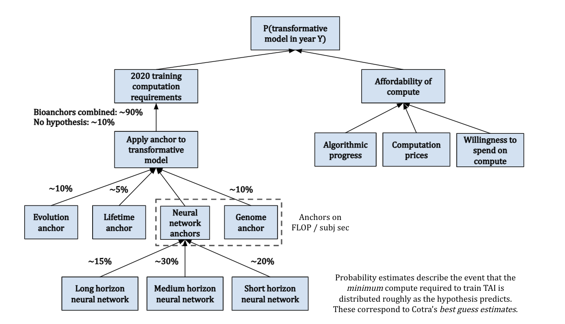
In calculating the training compute requirements distribution, Cotra places 90% weight collectively across these bioanchor hypotheses, leaving 10% to account for the possibility that all of the anchors significantly underestimate the required compute.
Here’s a visual representation of how Cotra breaks down the question “How likely is the development of TAI by a given year?”:
The above was essentially a summary of Cotra’s factorization of the question of AI timelines; for a summary of her key findings, see here.
Motivation
One of the biggest unresolved debates in AI Safety is the question of AI Timelines – when will Transformative AI (TAI) be developed? In 2020, Ajeya Cotra released a draft report, Forecasting TAI with biological anchors (Cotra, 2020), that aims to answer this question. It’s over 200 pages long including the appendices, and still just a draft!
Anecdotally, the results from this report have already been used to inform work in AI governance, and I believe it is likely that the report has had a major influence on the views of many researchers in AI safety.2 That said, the length of the document likely means that few people have read the report in full, are aware of its assumptions/limitations, or have a high-level understanding of the approach.
The aim of this post is to change this situation, by providing yet another summary of the report. I focus on the intuitions of the model and describe the framework visually, to show how different parts of Cotra’s report are pieced together.
Why focus on compute?
As you might imagine, trying to forecast the trajectory of a future transformative technology is very challenging, especially if there haven’t been many technologies of a similar nature in the past. In order to gain traction, we’ll inevitably have to make assumptions about what variables are the most important.
In the report, Cotra focuses on answering the following question:
In which year might the amount of computation required to train a “transformative model” become attainable for an AI development project?
Here, “transformative model” refers to a single AI model such that running many copies of that model (once trained) would have “at least as profound an impact on the world’s trajectory as the Industrial Revolution did”.3 It is a specific way that “transformative AI” could look – so Cotra’s report is essentially asking when we might have enough of a certain kind of resource (compute) to produce TAI through a certain path (training a giant AI model). She hopes that this sheds light on the broader question of “when might we have transformative AI” overall.
The question Cotra asks is thus more specific, but it seems plausibly informative for the broader question of TAI timelines because:
- The “train a big model” path to TAI seems technologically possible, and is salient because it’s similar to how current state-of-the-art AI systems are produced. (Indeed it’s an unusually brute-force approach to AI, so the question “When might we get TAI by training a single big model?” could be seen as a “soft upper bound” for the question of “When might we get TAI?”).
- It seems very plausible that compute is the resource that bottlenecks being able to train a transformative model the most. For instance (among other reasons):
- Many algorithms/architectures that saw success after the advent of Deep Learning had been proposed decades earlier, and only achieved competitive performance when researchers gained access to more compute
- Compute has been growing massively (by a factor of 10 billion times since 2010), compared to algorithmic efficiency, which has grown a comparatively small amount (44x since 2012)
- Evidence in favour of The Scaling Hypothesis and scaling laws suggest that there are regular and predictable returns to training AI models on increasingly large scales of compute
It’s also convenient that compute is relatively easy to measure compared to nebulous terms like “data” and “algorithms”, which lack standardised units. A common measure for compute is in terms of the total number of arithmetic operations performed by a model, measured in FLOP. We might also be interested in how many operations the model performs each second (measured in FLOP/s), which tells us about the power of the hardware that the model is trained on.
Framework
Cotra thus makes compute a primary focus of her TAI forecasting framework. Now instead of asking “when will TAI be developed?”, we ask two separate questions:
- 2020 training compute requirements: How much compute will we need to train a transformative model, using 2020 machine learning architectures and algorithms?
- Affordability of compute: How likely is it that we’ll be able to afford the compute required to train a transformative model in a particular year?
The second of these is relatively straightforward to answer because we have some clear trends that we can analyse and directly extrapolate.4 The first question however, opens a big can of worms – we need to find some kind of reference class that we can anchor to.
For this, Cotra chooses to anchor to the human brain – she views the human brain as a “proof of concept” that general intelligence is possible, then takes the analogy very seriously. The assumption is that the compute required to “train” the human brain should be informative of how much compute is needed to train a transformative model.
But how do we even define “compute to train the human brain”? There seem to be two main ambiguities with defining this:
- How long was the human brain “trained” for?
- For instance, should we interpret the brain as being trained for a human lifetime, or over the course of neuron evolution?
- How much compute was used at each point in training?
- For example, how many FLOP/s does the human brain run on?
Our answers to these questions determine the biological anchors – four5 possible answers to the question, “how much compute was used to train the human brain?”. Two of these anchor directly to FLOP of compute:
- Evolution anchor: The compute required to train a transformative model is roughly the total compute done over evolutionary history, starting from the first neurons. This interprets evolution as a really big search algorithm over a large space of possible neural architectures and environments, eventually stumbling across the human brain.
- Lifetime anchor: The compute required to train a transformative model is roughly the compute performed as a child matures, from birth to 32 years old. Under this hypothesis, we should expect machine learning architectures to be roughly as efficient as human learning.
The other two hypotheses anchor to the computations per second (i.e. FLOP/s) performed by the brain, rather than total compute. This is used to estimate the FLOP per subjective second (FLOP / subj sec) that TAI performs, where a “subjective second” is the time it takes a model to process as much data as a human can in one second.6 These hypotheses differ in how many parameters they predict TAI would need to have.
- Neural network anchors7: TAI should perform roughly as many FLOP / subj sec as the human brain, and have a similar ratio of “parameters” to “FLOP / subj sec” as today’s neural networks do. There are actually three anchors here, as we’ll later see.
- Genome anchor: TAI should perform roughly as many FLOP / subj sec as the human brain, and have about as many parameters as there are bytes in the human genome.
We can think of these anchors as saying that to build TAI, we’ll need processing power as good as the human brain, and as many parameters as (1) would be typical of neural networks that run on that much processing power, (2) the human genome.
You can see Cotra’s bioanchors framework at a high-level below:

On the left, we use bioanchors to determine how much compute we’ll need to train TAI. Overall, Cotra allocates 90% weight to the bioanchors, where the remaining 10% is reserved for the possibility that all of the hypotheses are significantly underestimating required compute. On the right, we do projections for when we’ll be able to afford this compute, based on trends affecting compute prices and the willingness to spend. These are combined to give an estimate for the probability of TAI by a particular year.
We saw earlier that the predicted FLOP for the evolution and lifetime anchors can be directly estimated, but this is not the case for the genome and neural network anchors. For this, we need to know both the number of FLOP / subj sec performed by the human brain, and the relevant number of subjective seconds required for training.
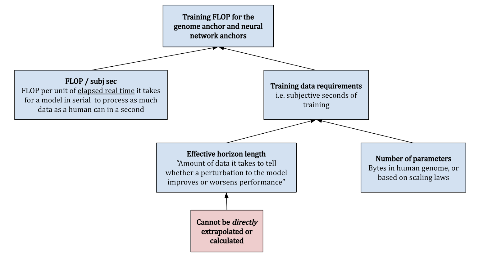
Finding the training data requirements is split into two parts:
- Number of parameters, which is specified by the relevant bioanchor hypothesis
- Effective horizon length – roughly, the amount of data it would take to tell whether a perturbation to the model improves or worsens performance.8 This is tricky to determine because it can’t be directly extrapolated or calculated making it one of the biggest uncertainties in the report.
Combining all of these gives us a rough estimate for the compute that the relevant bioanchor predicts.
You now know the basic motivation and framework for how the model works! The next section will dive into where a lot of the complexity lies – figuring out probability distributions over training compute for each of the bioanchors.
Zooming Into the Biological Anchors
We can think of each bioanchor as going through a three-step process:
- Find a prior distribution for the FLOP based on biological evidence
- Make adjustments based on evidence from current machine learning and intuitions
- Decide how strongly you want to weigh the anchor
In this section I’ll briefly outline9 the bioanchor hypotheses – I’ve also included a dependency diagram for each of them, where the boxes link to the relevant part of the report.
Evolution anchor
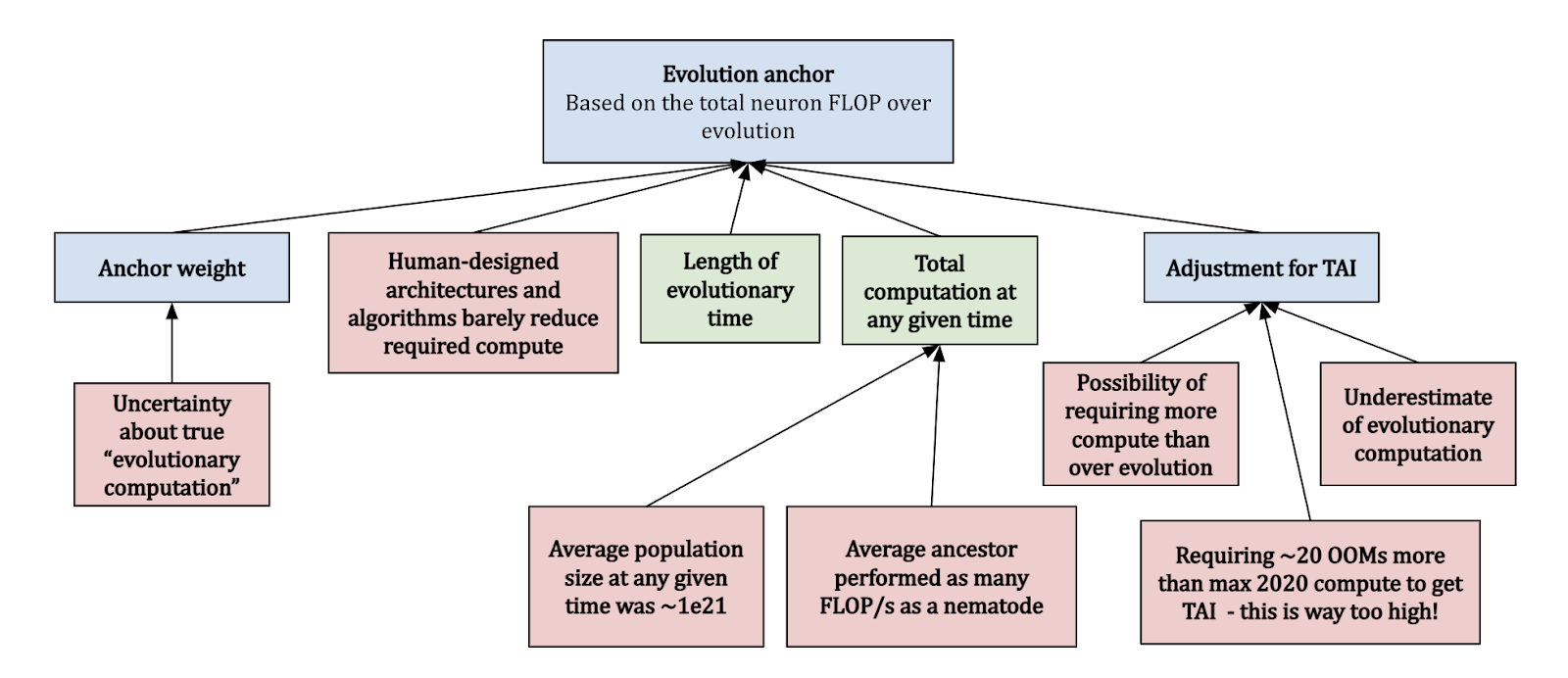
The evolution anchor looks at the total FLOP performed over the course of evolution, since the first neurons. Clearly there are some uncertainties with this approach:
- How do you even count “evolutionary computation”, and how does this compare with FLOP done on a GPU?
- What was the “average” compute done over all species at any time?
- How does the compute efficiency of human-designed architectures compare with just doing a random search?
Cotra accounts for these considerations, and assumes that the “average ancestor” performed as many FLOP/s as a nematode, and that there were on average ~1e21 ancestors at any time. This yields a median of ~1e41 FLOP, which seems extraordinarily high compared to modern machine learning.10 She gives this anchor a weight of 10%.
Lifetime anchor
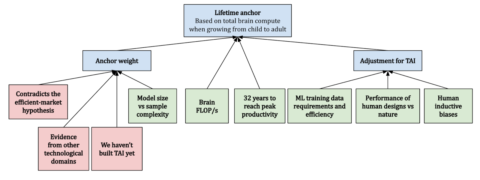
The second approach based on counting FLOP directly is based on the lifetime anchor, which looks at the total brain compute when growing from child to an adult (32 years old). Plugging in the numbers about brain FLOP/s seems to suggest that ~1e27 FLOP would be required to reach TAI. This seems far too low, for several reasons:
- Examples from other technological domains suggests that the efficiency of things we build (on relevant metrics) is generally not great when compared to nature
- It also contradicts the efficient-market hypothesis, and predicts a very substantial probability that AlphaStar-level compute would be TAI, which doesn’t seem to be the case!
Overall, Cotra finds a median of ~1e28 FLOP, and places 5% weight on this anchor.
Both the evolution and lifetime anchors seem to be taking a similar approach, but I think it’s really worth emphasising just how vastly different these two interpretations are in terms of their predictions, so here’s a diagram that illustrates this:
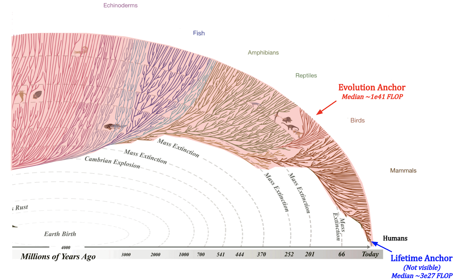
Image source: (For the evolutionary tree) evogeneao Tree of Life Explorer
If we look at the part of the evolutionary tree with neurons, then the evolution anchor includes neuron compute over the entire red area, across many different branches. On the other hand, the lifetime anchor requires us to zoom in really close to a small region in the bottom right, consider only humans out of all mammals, and consider only 32 years of the life of a single human out of the ~100 billion people who’ve ever lived. This isn’t even close to being visible in the diagram11!
Neural network anchors
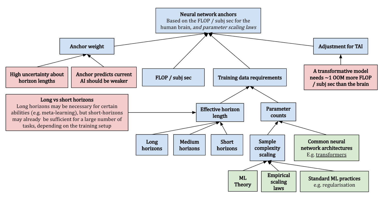
The three neural network anchors look at how much compute is required to train a network, by anchoring to the FLOP / subj sec performed by the brain, and based on parameter scaling laws. These anchors differ based on what horizon length is seen as necessary to achieve transformative impacts, and each have their own corresponding log-uniform distribution.
- Short horizon: 1 subj sec to 1e3 subj sec, centred around ~1e32 FLOP
- Medium horizon: 1e3 subj sec to 1e6 subj sec, centred around ~3e34 FLOP
- Long horizon: 1e6 subj sec to 1e9 subj sec, centred around ~1e37 FLOP
Cotra determines the training data requirements based on a mix of machine learning theory and empirical considerations. She puts 15% weight on short horizons, 30% on medium horizons, and 20% on long horizons, for a total of 65% on the three anchors.
Genome anchor
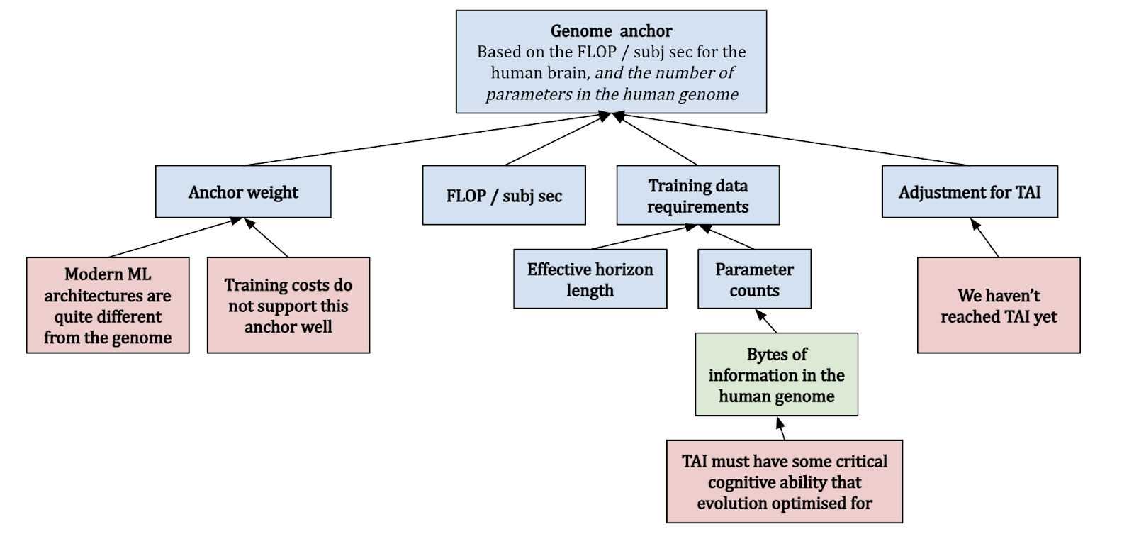
The genome anchor looks at the FLOP / subj sec of the human brain, and expects TAI to require as many parameters as there are bytes in the human genome. This hypothesis implicitly assumes a training process that’s structurally analogous to evolution12, and that TAI will have some critical cognitive ability that evolution optimised for.
At least at the time of writing (May 2022), machine learning architectures don’t look very much like human genome, and we are yet to develop TAI – thus Cotra updates against this hypothesis towards requiring more FLOP. Overall, she finds a median of ~1e33 FLOP and places 10% weight on this anchor.
Affordability of compute
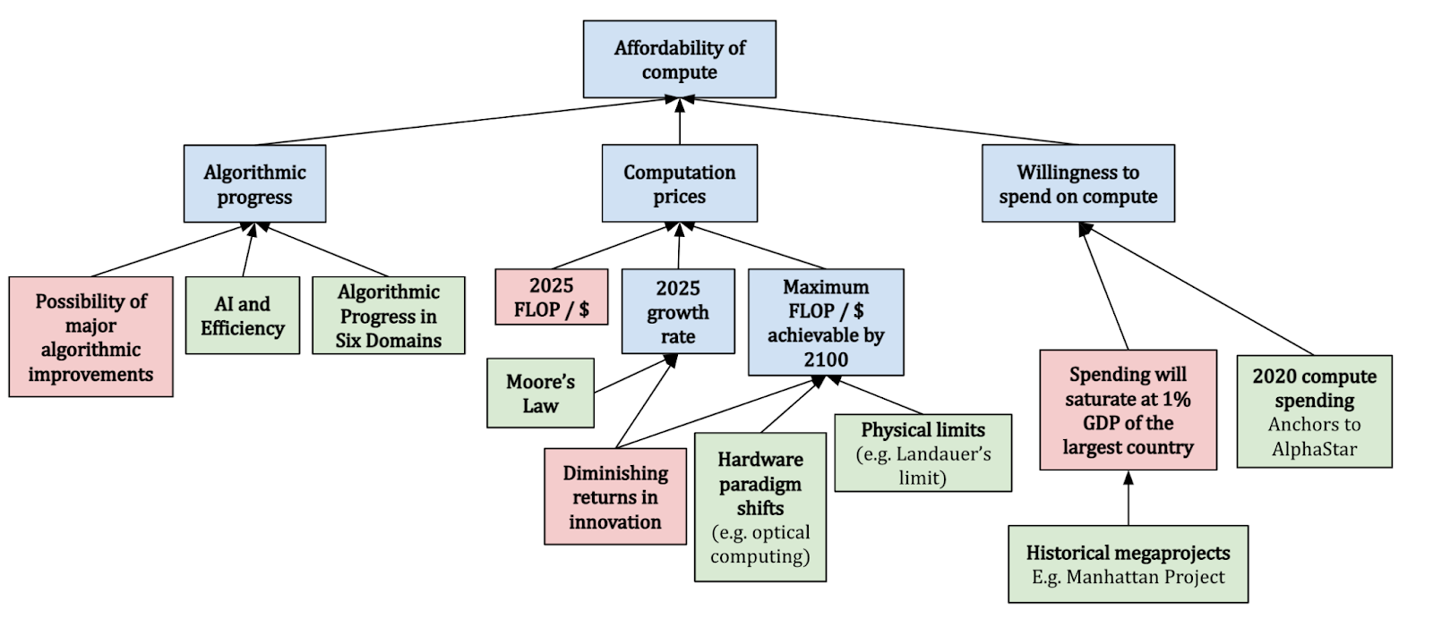
After using the bioanchors to determine a distribution for the compute FLOP required to build TAI using 2020 algorithms and architectures, Cotra turns to find a probability distribution over whether or not we’ll be able to afford this compute. She does this by considering three different factors:
- Algorithmic progress: For this, she relies heavily on the AI and Efficiency study, which finds a 44x growth in algorithmic efficiency for Computer Vision algorithms between 2012 and 2018. She considers a doubling in efficiency every ~2-3 years, although the cap on progress depends on the specific bioanchor hypothesis
- Computation prices: We should expect to get more compute for a given price over time – Cotra bases this roughly on current trends in compute prices; halving every ~2.5 years, and further expects this to level off after 6 orders of magnitude.
- Willingness to spend: Cotra assumes that the willingness to spend on machine learning training runs should be capped at 1% the GDP of the largest country, referencing previous case studies with megaprojects (e.g. the Manhattan Project), and should follow a doubling time of 2 years after 2025.
She makes these forecasts starting from 2025 to 2100, because she believes that there will be a rapid scaleup in compute for ML training runs from 2020 to 2025, and expects this to slow back down. The main uncertainty here is whether or not existing trends are going to persist more than several years into the future. For instance, we (Epoch AI) recently found that OpenAI’s AI and Compute investigation was too aggressive in its findings for compute growth. In fact, there is evidence that the reported trend was already breaking at the time of publishing. All in all, I think this suggests that we should exercise caution when interpreting these forecasts.
Putting Things Together: Final distribution
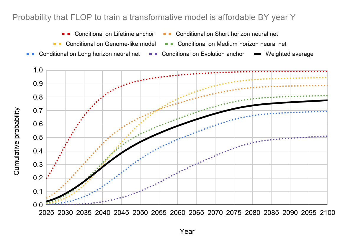
If we put everything together, this is the distribution that we get:
P(TAI before 2030) | P(TAI before 2050) | P(TAI before 2100) |
~8% | ~47% | ~78% |
10% | 50% | 90% |
2031 | 2052 | >2100 |
Based on these results, Cotra chooses a median estimate of TAI by 2050, a round number that avoids signalling too much precision in the estimates. These results seem to suggest that the probability of TAI being developed within this century is very high (at ~78%, see the table above).
You can of course question the premises and approach of this study, for instance:
- Is compute actually the biggest factor driving AI developments? Is it really reasonable to think of this as the main bottleneck, even a decade into the future?
- How valid is the approach of using bioanchors to determine the required compute to train TAI13?
- The report ignores the possibility of new paradigms (e.g. optical computing) and exogenous events that could hamper development – how much should we still trust this model?
Among other sources, Cotra states that the largest source of uncertainty comes from the appropriate value of the effective horizon length, which could range from 1 subj sec to 1e9 subj sec in the neural network anchors, and states that this is subject to further investigation. She also argues that the model overestimates the probability of TAI for short timelines due to unforeseen bottlenecks (e.g. regulation), and underestimates it for long timelines, since the research field will likely have found different paths to TAI that aren’t based on scaling 2020 algorithms and architectures.
Conclusion
All in all, this is one of the first serious attempts at making a concrete framework for forecasting TAI, and it’s really detailed! Despite this, there are still tons of questions that remain unanswered, that hopefully the AI forecasting field can figure out soon enough.
I also hope that these diagrams and explanations help you get a good high-level overview of what the report is getting at, and what kinds of further work would be interesting! You can find the full report and code here, which I encourage you to look through.
You can play with the diagrams here (the boxes link to the corresponding part of the report). These were rather clunkily put together using Google Slides – if you have any suggestions for better software that’s good for making these diagrams, I’d love to hear it!
Notes
-
Green boxes correspond to inputs, red boxes are assumptions or limitations, and blue boxes are classed as “other”.
-
By “AI Safety”, I am referring generally to work that helps reduce global catastrophic risks from advanced AI systems, which includes both AI governance and technical AI safety.
-
In general, it is not necessarily the case that these transformative effects need to be precipitated by a single model, although making this assumption is arguably still a good proxy for when we might see transformative impacts from multiple AI systems. The report also gives a more precise definition of “impact” in terms of GWP, but my impression is that the heavy lifting assumption-wise is done by the bioanchors, rather than the precise definition of TAI. That is, I suspect the same bioanchors would’ve been used with somewhat different definitions of TAI.
-
Of course, things aren’t quite so straightforward! For instance, we also need to consider the possibility of trends failing to persist, e.g. due to the end of Moore’s Law.
-
In her report, Cotra gives the following example: “a typical human reads about 3-4 words per second for non-technical material, so “one subjective second” for a language model would correspond to however much time that the model takes to process about ~3-4 words of data. If it runs on 1000 times as many FLOP/s as the human brain, but also processes 3000-4000 words per second, it would be performing about as many FLOP per subjective second as a human.”
-
Since the neural network anchors don’t really correspond to any biological process, an alternative and arguably more accurate framing for them is “how much compute would it take to train a model as good as the human brain?” (as opposed to “how much compute was required to train the human brain?”).
-
For instance, for a True or False question answering task given a sentence, the effective horizon length might be the length of the input sentence.
-
My goal here is to provide a succinct summary of the key points, and to simultaneously provide links for people who want to learn more, so I refrain from putting too much detail here.
-
E.g. Google’s PaLM model was trained with ~2.5e24 FLOP – that’s 17 orders of magnitude smaller!
-
Of course, this diagram doesn’t account for the fact that certain species do a lot more compute than others, but I think it gets some intuition across – that there’s a great deal of uncertainty about how much compute was required to “train” the human brain.
-
This differs from the evolution anchor in that it assumes we can search over possible architectures/algorithms a lot more efficiently than evolution, using gradients. Due to this structural similarity, and because feedback signals about the fitness of a particular genome configuration are generally sparse, this suggests that the anchor only really makes sense with long horizon lengths. This is why there aren’t also three separate genome anchors!
-
In my view, this is the perspective that Eliezer Yudkowsky is taking in his post, Biology-Inspired AGI Timelines: The Trick That Never Works. See also Holden Karnofsky’s response.

