Summary
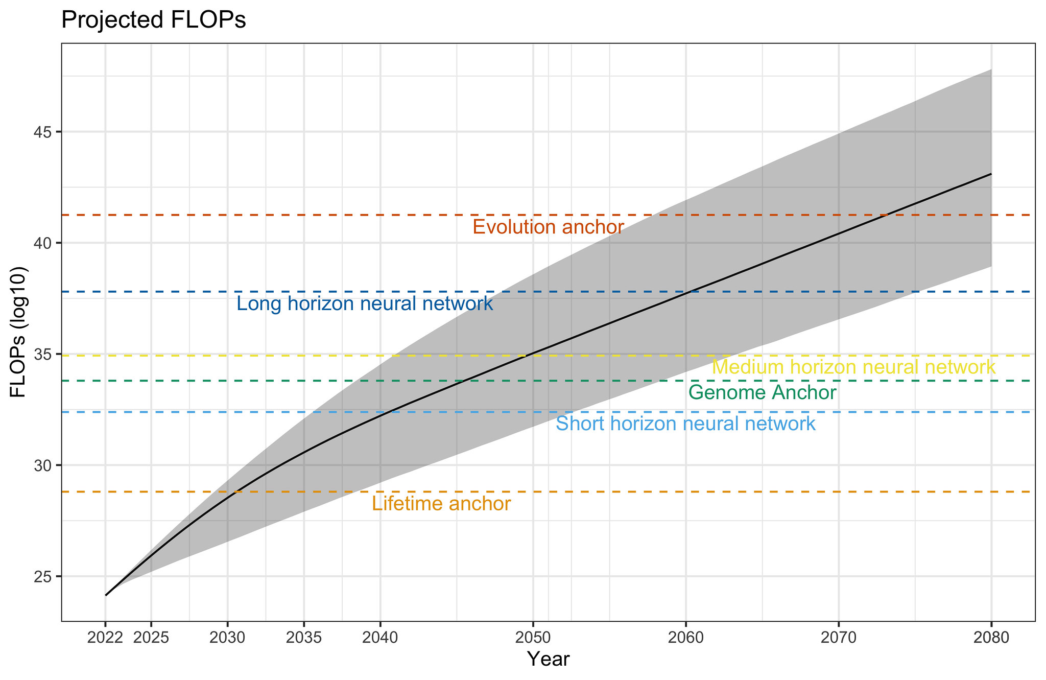
Using our dataset of milestone machine learning models, and our recent analysis of compute trends in ML, we project forward 70 years’ worth of trends in the amount of compute used to train machine learning models. Our simulations account for (a) uncertainty in estimates of the growth rates in compute usage during the Deep Learning (DL)-era and Pre-DL era, and (b) uncertainty over the ‘reversion date’, i.e. the date when the current DL-era compute trend (with a ~6 month doubling time) will end and revert to the historically more common trend associated with Moore’s law. Assuming a reversion date of between 8 to 18 years, and without accounting for algorithmic progress, our projections suggest that the median of Cotra 2020’s biological anchors may be surpassed around August 2046 [95% CI: Jun 2039, Jul 2060]. This suggests that historical rates of compute scaling, if sustained briefly (relative to how long these trends have been around so far), could result in the emergence of transformative models.
Our work can be replicated using this Colab notebook.
Note: we present projections, not predictions. Our post answers the question of: “What would historical trends over the past 70 years when naively extrapolated forward imply about the future of ML compute?” It does not answer the question: “What should our all-things-considered best guess be about how much compute we should expect will be used in future ML experiments?”
Introduction
Recently, we put together a dataset of over a hundred milestone machine learning models, spanning from 1952 to today, annotated with the compute required to train them. Using this data, we produce simple projections of the amount of compute that might be used to train future ML systems.
The question of how much compute we might have available to train ML systems has received some attention in the past, most notably in Cotra’s Biological Anchors report. Cotra’s report investigates TAI timelines by analyzing: (i) the training compute required for the final training run of a transformative model (using biological anchors), and (ii) the amount of effective compute available at year Y. This article replaces (ii) the compute estimate by projecting 70 years’ worth of trends in the amount of compute used to train machine learning models.
Cotra’s amount of effective compute available at year Y is broken down into forecasts of (a) compute cost, (b) compute spending, and (c) algorithimic progress. By contrast, we do not decompose the estimate, and rather project it on our previous investigation of training compute of ML milestone systems. This trend includes the willingness to spend over time including the reduced compute costs over time; however, it does not address algorithmic progress. We explicitly do not forecast the cost of compute or compute spending.
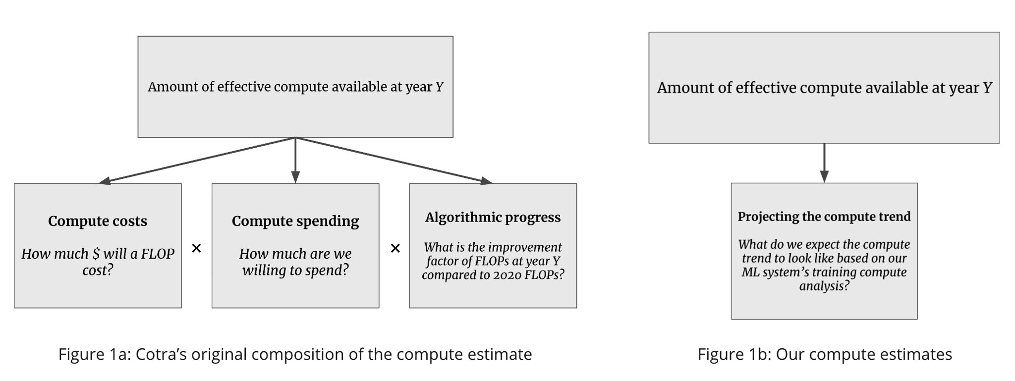
Figure 1. Contrasting our work with that of Cotra 2020
In this post, we present projections based on previously observed trends and some basic insights about how long the current 6-month doubling time can be sustained. That is, our post answers the question of: what would current trends imply about the future if you naively extrapolate them forwards.
One key reason we don’t expect these projections to be particularly good predictions is that it seems likely that Moore’s law might break down in some important way over the next few decades. We therefore might expect that that the doubling-time in compute usage, when the dollar-budgets to scale compute grow at the economic growth-rate, will be substantially longer than the historically common ~20-month doubling period.
When will the current scaling trend revert back to Moore’s law?
In our recent analysis of compute trends in ML (Sevilla et al., 2022), we find that, since the advent of Deep Learning, the amount of compute used to train ML systems has been doubling every 6 months. This is much faster than the previous historical doubling time that we find to be roughly 20 months (which is roughly in line with Moore’s law). Previous work (Carey, 2018, and Lohn and Musser, 2022) has pointed out that a scaling-rate that outstrips Moore’s law by a wide margin cannot be sustained for many years as a rate of growth in ML compute spending that far exceeds economic growth cannot be sustained for many years.
A key question, then, for projecting compute used in future ML systems, is: How long can the current fast trend continue, before it reverts to the historically much more common trend associated with Moore’s law?
To answer this question, we replicate the analysis by Carey, 2018, but instead of using the numbers from OpenAI’s AI and Compute (Amodei and Hernandez, 2018), we use the numbers from our recent analysis (summary).1 This analysis, roughly, points to three scenarios:
- Bearish: slow compute cost-performance improvements and very little specialized hardware improvements. In this scenario, it takes 12 years for the cost of computation to fall by an OOM. The current 6-month doubling period can be maintained for another ~8 years.
- Middle of the road: Moderate compute cost-performance improvements and moderate improvements in specialized computing. In this scenario, it takes roughly 7 years for the cost of computation to fall by an OOM, and progress in specialized hardware helps sustain the trend ~3 additional years. The current 6-month doubling period can be maintained for another ~12 years.
- Bullish: Fast compute cost-performance improvements and substantial improvements in specialized computing. In this scenario, it takes 4 years for the cost of computation to fall by an OOM, and progress in specialized hardware helps sustain the trend ~6 additional years. The current 6-month doubling period can be maintained for another ~18 years.
Roughly, we might say that these scenarios are represented by the following distributions over ‘reversion dates’, i.e. dates when the scaling trends are more similar to Moore’s law than they are to the current fast trend.
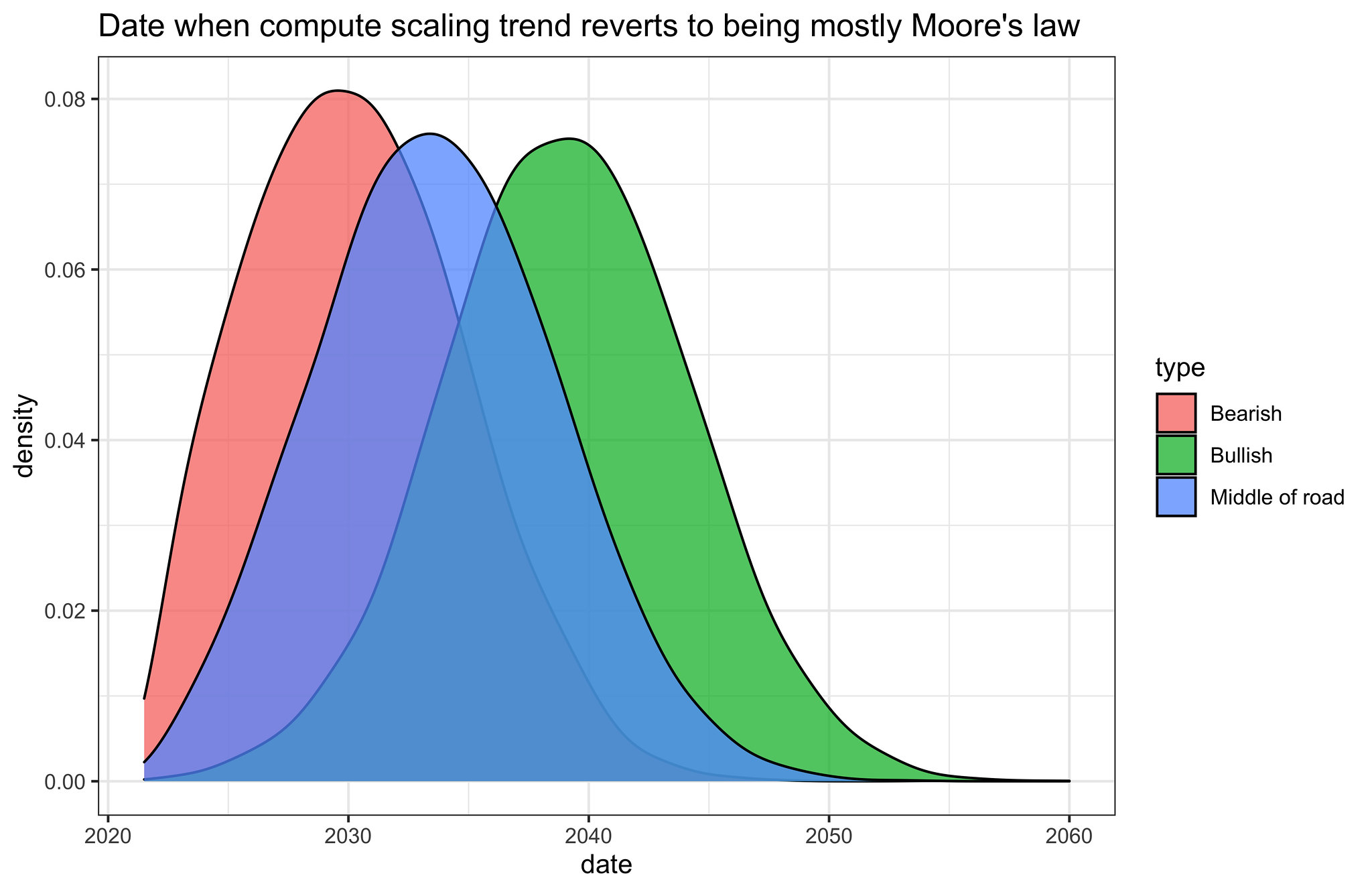
Fig 2. Distributions that roughly correspond to the three scenarios that come out of our replication of Carey, 20181
We then produce a mixture of these distributions by creating a weighted linear pool where “Bearish” is assigned 0.75, “Middle of the road” is assigned 0.20, and “Bullish” 0.05, based on our best-guesses (you can apply your own weights using this Colab notebook.)
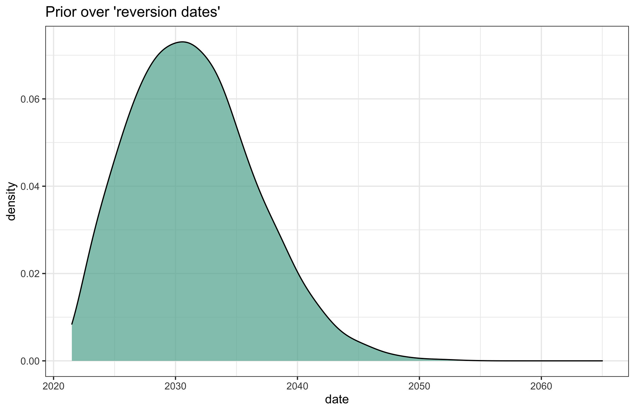
Fig 3. our best-guess for a prior over reversion dates, formed by mixing the previous distributions
We can use this as our prior over when the fast-trend will revert to the more historically common trend associated with Moore’s law.
Projecting ML compute trends
We simulate compute paths based on (a) our estimates of the growth rates in compute usage during the DL-era and Pre-DL era, and (b) our prior over ‘reversion date’, i.e. the date when the current DL-era compute trend will end. We account for the uncertainty in both (a) and (b) in our simulations (see details here).

Fig 4. 10,000 projected compute paths. Solid line represents the median projected compute at each date, and the shaded region represents 2-standard deviations around the median.
Our simulations reveal the following projections about the amount of compute used to train ML models.
| Year | Projected FLOP used to train largest ML model | Enough for how many anchor’s median compute requirements? |
|---|---|---|
| 2025 | \(10^{25.90}\) [\(10^{25.33}\), \(10^{26.14}\)] | 0/6 |
| 2030 | \(10^{28.67}\) [\(10^{26.71}\), \(10^{29.47}\)] | 0/6 |
| 2040 | \(10^{32.42}\) [\(10^{29.27}\), \(10^{34.71}\)] | 1/6 |
| 2050 | \(10^{35.26}\) [\(10^{31.78}\), \(10^{38.86}\)] | 3/6 |
| 2060 | \(10^{38.10}\) [\(10^{34.35}\), \(10^{42.49}\)] | 5/6 |
| 2070 | \(10^{40.79}\) [\(10^{36.83}\), \(10^{45.49}\)] | 5/6 |
| 2080 | \(10^{43.32}\) [\(10^{39.04}\), \(10^{48.18}\)] | 6/6 |
Table 1: Projected FLOP from 2025 to 2080
These projections suggest that, without accounting for algorithmic progress, the most modest of Cotra 2020’s biological anchors will be surpassed around August 2030 [95% CI: Jan 2029, May 2038], the median anchor (~\(10^{34.36}\) FLOP) will be surpassed around August 2046 [95% CI: Jun 2039, Jul 2060], and the strongest of anchors will be surpassed around May 2072 [95% CI: Jan 2057, Jun 2089].
Conclusion
If we naively extrapolate the trends uncovered from 70 years’ worth of compute scaling in machine learning, we find that within roughly 25 years, large-scale ML experiments will use amounts of compute that exceed the half of the compute budgets that Cotra 2020 has suggested may be sufficient for training a transformative model. This highlights the fact that historical rates of compute scaling in machine learning, even if sustained relatively briefly (relative to how long these trends have been around so far), could place us in novel territory where it might be likely that transformative systems would be trained. This work also suggests that understanding compute trends might be a promising direction for predicting ML progress.
Details of the simulations
We assume compute grows exponentially in time at some rate \(g\):
\[\begin{equation} C(t) = C(0) e^{gt}, \hspace{0.15cm} \text{where} \hspace{0.15cm} t \geq 0. \end{equation}\]In our projections, we replace \(g\) with \(g^*\), defined as a weighted geometric mean of our best-guess of the growth rate during Moore’s law (\(\tilde{g}_{\text{M}}\)), and the growth rate of our estimate of the growth rate during the Deep-Learning Era (\(\hat{g}_{\text{DL}}\)):
\[\begin{equation} g^* = \hat{g}_{\text{DL}}^{w(t)} \tilde{g}_{\text{M}}^{1-w(t)}, \hspace{0.15cm} \text{where} \hspace{0.15cm} w(t) \in [0,1]. \end{equation}\]Here, \(\hat{g}_{\text{DL}}\) simply denotes the growth rate during the Deep Learning Era (2010 onwards) as estimated using OLS. In particular, we estimate the following model using our dataset:
\[\begin{equation} \log C(t) = \beta + g_{DL}t, \hspace{0.15cm} \text{where} \hspace{0.15cm} t>2010. \end{equation}\]\(\tilde{g}_{\text{M}}\) is defined as follows:
\[\begin{equation} \tilde{g}_{\text{M}} = \sqrt{\hat{g}_{\text{M}}g_{\text{20-month}}}, \end{equation}\]where \(\hat{g}_{\text{M}}\) is the estimated growth rate during the Pre-DL era, and \(g_{\text{20-month}}\) is the growth rate implied by a 20-month doubling period. The reason we take the geometric mean of the estimated growth rate, and the growth rate implied by a 20-month doubling period is because Moore’s law is sufficiently well-established that the error bars around \(\hat{g}_{\text{M}}\) are too large relative to how well-established Moore’s law is. We therefore artificially increase our precision of the growth rate associated with Moore’s law by taking an average of our estimated value and the usual growth rate implied by an ~20-month doubling-time.
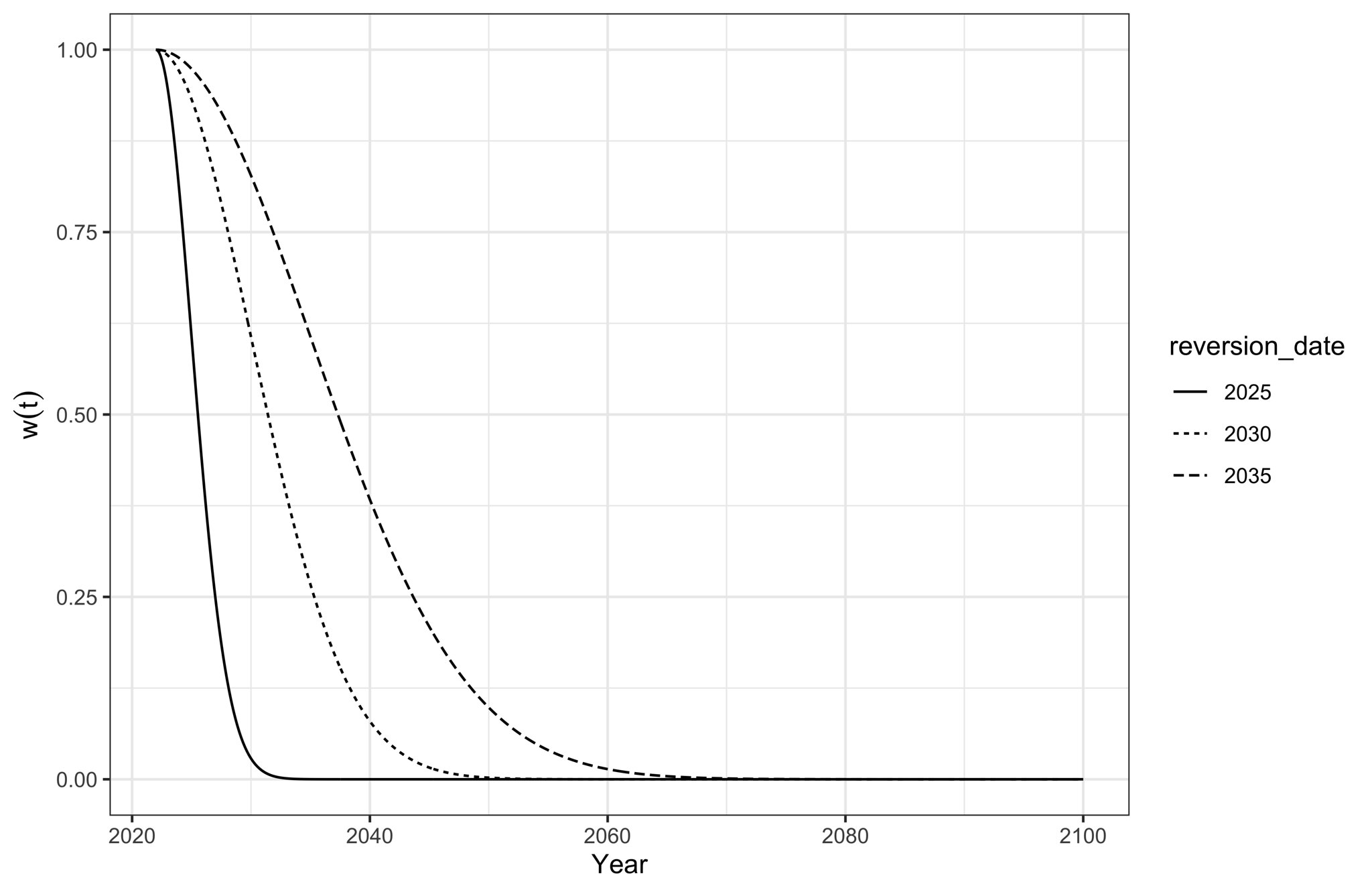
Our weight function, \(w(t)\), is constructed as follows:
\[\begin{equation} w(t) = \exp\bigg(\frac{(t-2022)^2}{2(\text{reversion date}-2022)^2}\bigg)^{-1}. \end{equation}\]Why? Well, it’s a logistic-like function with a unit-interval range, which exceeds \(1/2\) when \(t< \text{reversion date}\), equals \(1/2\) when \(t = \text{reversion date}\), and is less than \(1/2\) otherwise. This is what it looks like:
We then simulate some path \(C^j\) as follows:
\[\begin{equation} C_j = C(2022) e^{g^*_{j}t}, \hspace{0.15cm} \text{where, for any } \hspace{0.15cm} j: \end{equation}\]- \(\hat{g}_{\text{DL}}\) is estimated on our randomly sampled (with replacement) DL-Era Data,
- \(\hat{g}_{\text{M}}\) is estimated on our randomly sampled (with replacement) Pre-DL Era data, and
- \(w(t)\) is set based on a randomly sampled reversion date from our prior over reversion dates.
Notes
About the authors


