Introduction
A significant advantage of AI models over human intelligence is the ability to train a model once and then serve arbitrarily many copies of it for inference. This ‘train-once-deploy-many’ property means we can justify spending far more resources to train a single AI model than we could ever spend training a single human (something that AI labs have recently started doing). For example, it’s common for frontier models to be trained on tens of thousands of GPUs, yet each instance during inference requires only a few dozen GPUs.
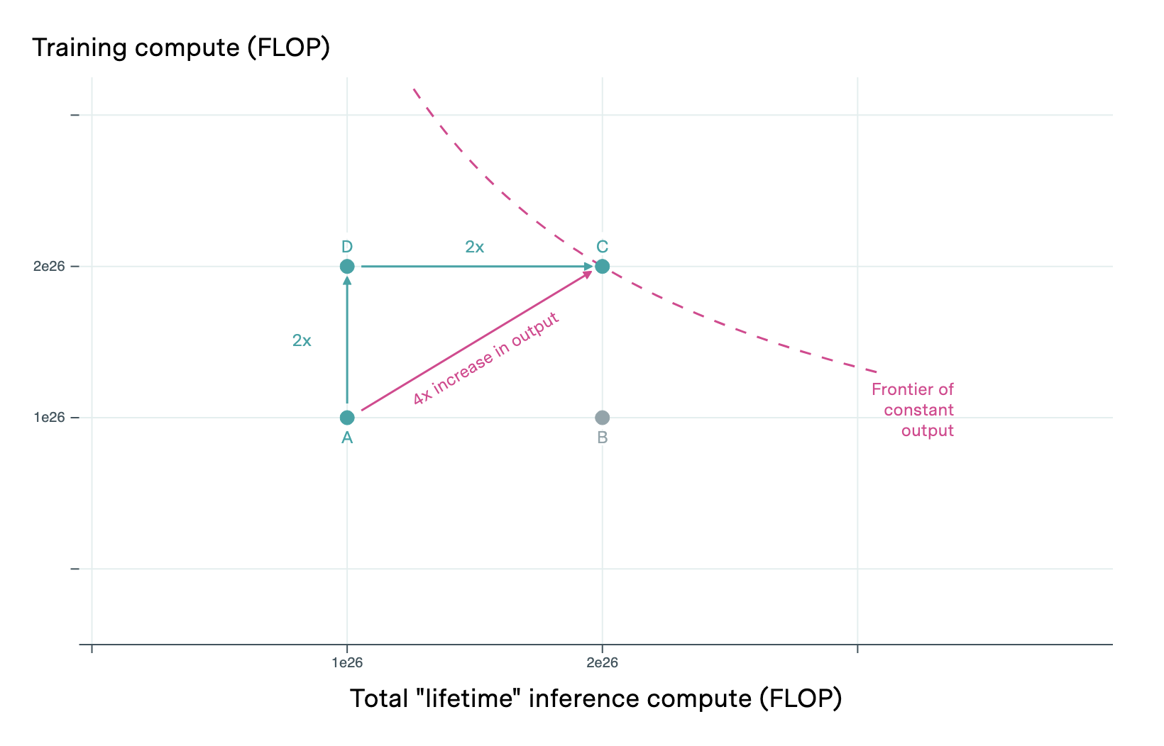
This difference suggests that AI systems exhibit increasing returns to scale when we add more compute for training and inference. If we set aside price effects for the moment, then with twice the compute, we can double economic output simply by running twice as many copies of the models we’re using for inference. In addition, we can use the same extra compute to train models using twice the training compute, and we expect these larger models to be more efficient at converting inference compute into output. By doing both—deploying more copies and improving their efficiency—our total economic output grows by more than double. We discuss later how rising AI output may also affect prices and dampen these gains, but under the simplifying assumption of stable prices, this potential for more-than-linear scaling remains clear.
This mechanism parallels how R&D creates increasing returns in the broader economy. For example, a similar argument can be made for why the R&D and technological progress leads to increasing returns to scale in human economies: twice the people and capital inputs means twice the output using current technology, but twice the number of researchers and economic activity also speeds up R&D, which increases the efficiency with which we use said resources. Consequently, the economic output increases by more than double, achieving a similar effect through a different mechanism as seen with AI systems.
The key difference is this: AI systems can benefit from both innovation and replication, whereas humans benefit only from innovation. The ‘train-once-deploy-many’ property of AI models creates a unique source of increasing returns that is unattainable with human workers. Hence, however compelling we find increasing returns to scale in the case of human economies, we should find them much more compelling in an economy where production is dominated by AI workers.
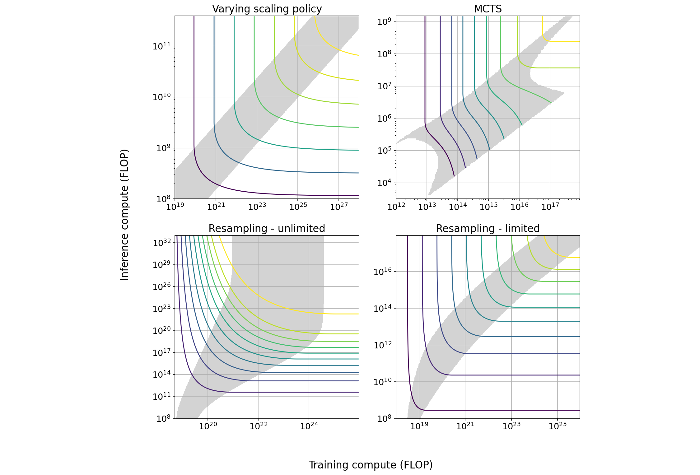
While increasing returns to scale being a consequence of the ‘train-once-deploy-many’ property of AI models seems plausible, it’s not immediately obvious how to quantify its magnitude. It turns out we can do this if we have estimates of the slope of the training-inference compute tradeoff, a subject explored in our prior work (here and here).
The core idea is that for many tasks done by AI models, it’s possible to reduce compute used at training time at the expense of increasing compute used at inference time (or vice versa) and maintain the same level of performance. The crucial parameter for our purposes turns out to be how many orders of magnitude of inference compute can we give up for each order of magnitude increase in training compute.
The basic argument
Say that \(f(T, I)\) is a production function that measures how much output an AI model can generate. Here, \(T\) represents the compute spent training the model, and \(I\) represents the compute spent running it. This output could be lines of code of a certain quality, or even research and development on GPU production - this latter case is important due to the feedback loops it enables, as we will see later.
We will demand two properties from our production function \(f\):
- Linear scaling with inference compute: For a fixed amount of training compute \(T\), doubling inference compute \(I\) should double output. Mathematically, this means \(f(T, I) = g(T) \cdot I\) for some function \(g(T)\). The intuition is that running twice as many copies of the same model should produce twice as much output.
- The training-inference compute tradeoff. For some constant \(c > 0\), we have that for all values of \(T\), \(I\) and \(x\), \(f(T, I) = f(T/x, I \cdot x^c)\). In other words, we can trade off 1 OOM of training compute for \(c\) OOMs of inference compute while maintaining the same output. Our prior work suggests values of \(c\) that are around 1, though with substantial uncertainty.
These two properties together determine the form of \(f\). If we set \(x = T\) in property 2, we get: \(f(T, I) = f(T/T, I \cdot T^c) = f(1, I \cdot T^c)\). Then using property 1, this equals \(g(1) \cdot I \cdot T^c\). So the output \(f\) must be proportional to \(I \cdot T^c\).
The fact that doubling our number of chips allows us to double both I and T gives us the increasing returns to scale we were looking to find, and the parameter c quantifies the magnitude of this increasing returns to scale.
Doesn’t this assume an infinite span for the tradeoff?
A key limitation of our model is that it assumes you can always trade more training compute for less inference compute (or vice versa) while maintaining performance. In practice, this tradeoff is limited—at some point, adding more of one type of compute cannot compensate for reducing the other type. Even when combining different methods for trading off compute, we typically only see tradeoffs spanning a few orders of magnitude.
Fortunately, we don’t need this tradeoff to work indefinitely to achieve increasing returns to scale. It’s sufficient if the tradeoff holds for values of \(T\) and \(I\) such that \(k_1 < T/I < k_2\), where \(k_1\) and \(k_2\) are constants with \(k_2 > k_1\). This scenario is much more plausible.
To see this, we iterate in a slightly more sophisticated way: letting \(h = (k_2 / k_1)^{1+c}\), we have:
\[ f(T, I) = \dfrac I T \cdot k_2 \cdot f\left(T, \dfrac T {k_2}\right) = \dfrac I T \cdot k_2 \cdot f\left(\dfrac T h, h^c \cdot \dfrac T {k_2}\right) \]\[ = \dfrac I T \cdot k_2 \cdot h^{ 1+c } \cdot f\left(\dfrac T h, \dfrac T { k_2 \cdot h } \right) \]\[ = h^{ 1+c } \cdot f\left(\dfrac T h, \dfrac I h\right) \]In other words, reducing both \(T\) and \(I\) by a factor of \(h\) reduces our total output by a factor of \(h^{1+c}\). This gives us exactly the increasing returns to scale we wanted, even when we keep the ratio of training to inference compute within fixed bounds.
In practice, we eventually expect this tradeoff to break down even inside a fixed cone. This is because for any good, we expect there to be a minimum level of compute necessary to produce one unit of that good: for example, we can’t produce an original token by something less than ~1 FLOP. If \(f\) were to represent the number of tokens that we could produce, then the implication of indefinite increasing returns to scale would be that with \(N\) chips we could produce ~\(N^a\) tokens per second for \(a > 1\), and so taking \(N\) sufficiently large we could lower the FLOP cost of producing each token below 1 FLOP, violating the aforementioned lower bound.
We can avoid this implausible conclusion by simply restricting our attention to the region of this cone where \(T\) is bounded from above by some constant, where the constant will in practice depend on the production of what good or service is being represented by the function \(f\). This roughly corresponds to saying that there is some training compute threshold over which we get no additional meaningful performance improvements on the task we’re focusing on. Then, the increasing returns to scale argument will work in this region per our argument above, and the final conclusion will be that we can get increasing returns to scale on our compute stock for some number of doublings before the training-inference tradeoff breaks down.
What does this imply about an AI-only economy?
Let’s explore a simplified economic model where AIs are advanced enough to manufacture computer chips. Intuitively, we might expect accelerating growth in such a scenario, and this expectation turns out to be correct.
For simplicity, the only capital good is computer chips, the stock of which is denoted by \(K\), and the production function \(f\) also represents the production of computer chips. Chips do not depreciate, and the economy allocates a fraction \(q\) of its chips to training and \(1-q\) to inference for some \(0 < q < 1\). Furthermore, we assume all output is reinvested to increase the stock of computer chips. In this case, we can write the equations describing the dynamics of this economy as follows:
\[ \frac{dK}{dt} = f(T, I) \sim I \cdot T^c = (1-q) \cdot K \cdot T^c \]\[ \frac{dT}{dt} = q \cdot K \]It’s easy to show that this economy will exhibit accelerating hyperbolic growth: informally, every time \(K\) doubles, we also get a doubling of \(T\), and this increases the growth rate of \(K\) by a factor of \(2^c\). We’ve previously analyzed the properties of these dynamical systems more rigorously in our work on explosive growth from AI, and we omit the detailed discussion here for the sake of brevity. Below, we give an example of what the system looks like when we use \(c = 1\), \(q = \frac{1}{2}\) and initial conditions \(T_0 = K_0 = 1\).

Figure 1. Plot of the compute stock \(K\) over time for \(q = \frac{1}{2}\), \(c = 1\), and initial conditions \(T(0) = K(0) = 1\). Note the log scale on the vertical axis: exponential growth would be a straight line, so \(K\) is growing super-exponentially as expected.
While the above toy model contains many unrealistic assumptions (output scales linearly with the number of AI workers, no depreciation of the compute stock, etc.) it illustrates an important principle: the ‘Train-Once-Deploy-Many’ nature of AI creates a strong tendency toward accelerating growth, as additional computer chips can be used both to run more copies of existing AI models and to train better ones.
About the authors


Related work