Notes:
- I give visual explanations for Tom Davidson’s report, Semi-informative priors over AI timelines, and summarise the key assumptions and intuitions
- The diagrams can be found here – you can click on some of the boxes to get linked to the part of the report that you’re interested in1
Thanks to the Epoch AI team for feedback and support! Thanks especially to Jaime Sevilla and Tom Davidson for providing detailed feedback.
Executive Summary
The framework in Semi-informative priors over AI timelines assumes a model of AGI development which consists of a sequence of Bernoulli trials, i.e. it treats each calendar year as a “trial” at building AGI with constant probability \(p\) of succeeding.
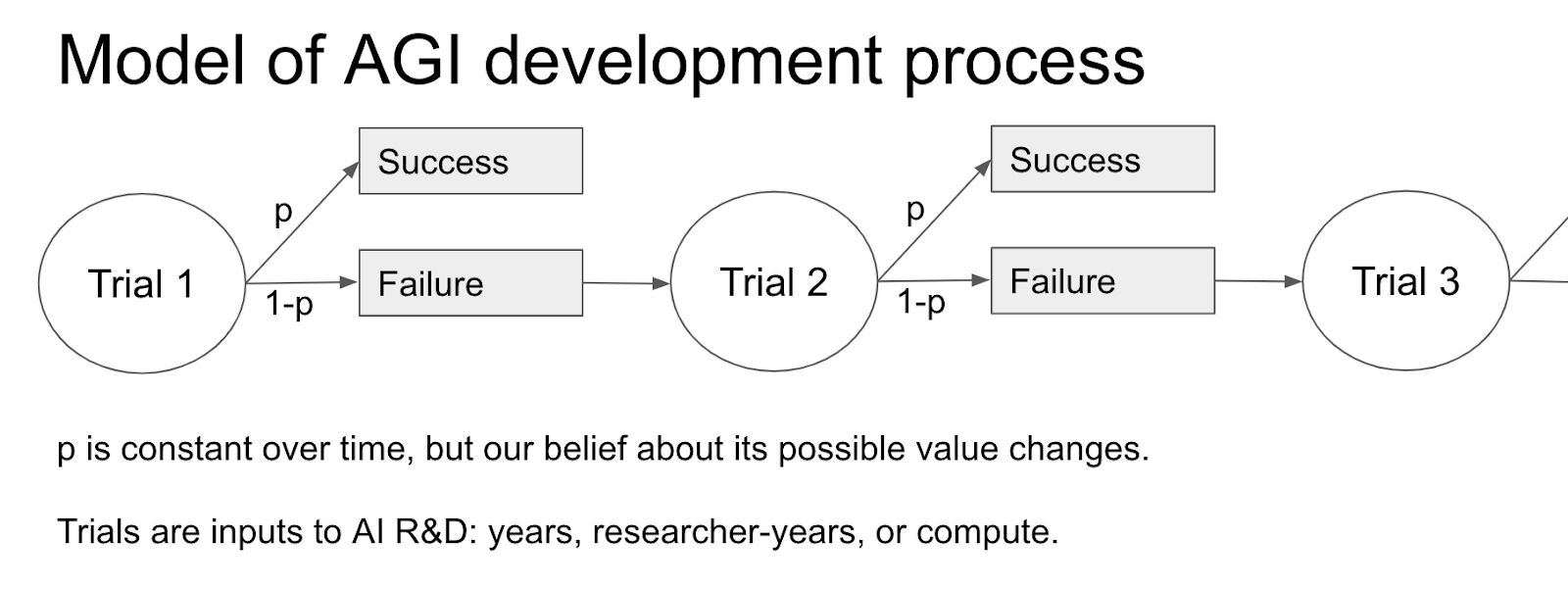
Image source: Davidson, 2021
However, we don’t know what this value of \(p\) is, so we use a generalisation of Laplace’s rule of succession to estimate \(P(\text{AGI next year} \mid \text{no AGI yet})\). This is done by specifying a first-trial probability, the probability of successfully building AGI in the first year of AI research, together with the number of virtual successes, which tells us how quickly we should update our estimate for \(P(\text{AGI next year} \mid \text{no AGI yet})\) based on evidence. The framework leans very heavily on the first-trial probability, which is determined using a subjective selection of reference classes (more here).
How much evidence we get depends on the number of trials that we see, which depends on the regime start-time – you can think of this as the time before which failure to develop AGI doesn’t tell us anything useful about the probability of success in later trials. For instance, we might think that 1956 (the year of the Dartmouth Conference) was the first year where people seriously started trying to build AGI, so the absence of AGI before 1956 isn’t very informative. If we think of each trial as a calendar year, then there have been 2021-1956 = 65 trials since the regime start-time, and we still haven’t developed AGI, so that’s 65 failed trials which we use to update \(P(\text{AGI next year} \mid \text{no AGI yet})\), where “next year” now corresponds to 2022 rather than 1957.
But why should a trial correspond to a calendar year? The answer is that it doesn’t have to! In total, Davidson considers three candidate trial definitions:
- Calendar-year trials: 1 trial = 1 calendar year
- Compute trials: 1 trial = a 1% increase in the largest amount of compute used to develop an AI system to date
- Researcher-year trials: 1 trial = a 1% increase in the total researcher-years so far
If we extend this reasoning, then we can predict the probability that AGI is built \(X\) years into the future. Davidson does this to predict \(P(\text{AGI by 2036} \mid \text{no AGI yet})\) as follows:
\[\begin{align}P(\text{AGI by 2036} \mid \text{no AGI yet}) &= 1-P(\text{no AGI by 2036} \mid \text{no AGI yet})\\&=1-P(\text{no AGI in 2022} \mid \text{no AGI by 2021})...P(\text{no AGI in 2036} \mid \text{no AGI by 2035}) \end{align}\]The idea is that this framework only incorporates a small amount of information based on observational evidence, giving “semi-informative priors” over AI timelines. This framework is shown in more detail below:
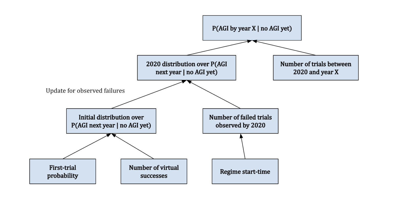
Since Davidson uses three different trial definitions, we actually get three of these diagrams!

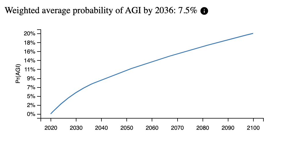
All in all, Davidson uses this to get a central estimate of \(P(\text{AGI by 2036} \mid \text{no AGI yet}) = 8\%\), with the following cumulative probability function:
Motivation
One way of forecasting AI Timelines is to consider the inner workings of AI, guess what kinds of developments are the most important, and then generate a probability distribution over when Artificial General Intelligence (AGI) will be developed. This is the approach taken by Ajeya Cotra in Forecasting TAI with biological anchors, a really detailed draft report that draws analogy to the human brain to forecast when Transformative AI (TAI) will first be developed. 2
Tom Davidson’s report, Semi-informative priors over AI timelines, is also a detailed report forecasting AI timelines, but it takes a different approach to Cotra’s report. Rather than thinking about the details of AI development, it assumes we know almost nothing about it3!
The goal of this post is to explain the model through the liberal use of diagrams, so that you can get high-level intuitions about how it works, hopefully informing your research or understanding of AI forecasting.
Laplace’s Rule of Succession
Suppose we’re trying to determine when AGI will first be developed, without knowing anything about the world except that there have been \(N\) years so far, and AGI has not been developed in any of these years. How would you determine the probability that AGI is developed in the next year4?
A naive approach we might take is to think of each year as a “trial” with two possible outcomes – (1) successful trials, where AGI is successfully built in the year of interest, and (2) failed trials, where AGI is not built in the year of interest. We then assume that the probability of building AGI in the next year is given by the total successful trials divided by the total trials:
\[P(\text{AGI next year} \mid \text{no AGI yet}) = \frac{\text{successes}}{\text{successes + failures}} = \frac{\text{successes}}{\text{total trials}}\]$$$$Since AGI hasn’t been built in any of the last \(N\) years, there have been zero successes out of \(N\) trials. We thus conclude that the probability of AGI in the next year is zero… but clearly there’s something wrong with this!
The problem is that this approach doesn’t even account for the possibility that AGI might ever be developed, and simply counting the number of successes isn’t going to be very helpful for a technology that hasn’t been invented yet. How can we modify this approach so that both the possibility of success and failure are considered?
One clever way of doing this is to consider “virtual trials”. If you know that it’s possible for each trial to be either a success or a failure, then it’s as if you had previously observed one “virtual success” and one “virtual failure”, which we can add to the total observed successes and failures respectively. We can then modify the equation to:
\[P(\text{AGI next year} \mid \text{no AGI yet}) = \frac{\text{successes + 1}}{\text{(successes + 1) + (failures + 1)}} = \frac{\text{successes + 1}}{\text{total trials + 2}}\]This equation is called Laplace’s rule of succession, which is one approach to estimating the probabilities of events that have never been observed in the past. In particular, it assumes that we know nothing about the world except for the number of trials and the number of successes or failures.
If we apply this method, then we find that the probability of building AGI in the next year is \(1/(N+2)\). Assuming that the field of AI was formed in 1956 at the famous Dartmouth Conference, then this suggests that \(N = 2021 - 1956 = 65\) and \(P(\text{AGI is built in 2022})=1/67\), or a probability of around 1.5%.
If we extend this reasoning, then we can predict the probability that AGI is built \(X\) years into the future. Davidson does this to predict \(P(\text{AGI by 2036} \mid \text{no AGI yet})\) as follows:
\[\begin{align}P(\text{AGI by 2036} \mid \text{no AGI yet}) &= 1-P(\text{no AGI by 2036} \mid \text{no AGI yet})\\&=1-P(\text{no AGI in 2022} \mid \text{no AGI by 2021})...P(\text{no AGI in 2036} \mid \text{no AGI by 2035}) \end{align}\]This seems a lot more reasonable than the naive approach, but there’s still some serious problems with it, like the following:
- It’s extremely aggressive before considering evidence: For instance, according to Laplace’s rule the attendants of the 1956 Dartmouth Conference should have predicted a 50% probability of developing AGI in the first year of AI research, and 91% probability within the first ten years!
- It’s sensitive to the definition of a “trial”: If we had chosen each trial to be “one day” instead of a year, our conclusions could be fairly different (more).
What’s going on here (among other things) is that the rule of succession makes very few prior assumptions – i.e. it’s an uninformative prior. In fact, it’s so uninformative that it doesn’t even capture the intuition that building a transformative technology in the first year of R&D is not commonplace! Clearly, we still need something better if we’re going to make predictions about AGI timelines.
Making the priors less uninformative
The solution that Davidson proposes is to make this prior less uninformative, by incorporating certain pieces of common sense intuition and evidence about AI R&D. Looking more closely at the framework given by Laplace’s rule of succession, we see that it depends on several factors:
- Regime start-time: You can think of this as the time before which failure to develop AGI doesn’t tell us anything useful about the probability of success in later trials. We’ve been assuming this to be 1956, but this doesn’t have to be the case!
- First-trial probability: The odds of success on the first “trial” from the regime start-time onwards
- Trial definition: Why are we using “one year” as a single trial, and what are some alternatives?
We can also add an additional modification, in the form of the number of virtual successes. This affects how quickly you update away from the first-trial probability given new evidence – the more virtual successes, the smaller your uncertainty about how difficult it is to build AGI, and thus the less you update based on observing more failed trials. For example, suppose that your initial \(P(\text{AGI next year} \mid \text{no AGI yet})\) is 1/100:
- If you start with 1 virtual success, then after observing 100 failed trials your updated \(P(\text{AGI next year} \mid \text{no AGI yet})\) is now 1/200
- In contrast, if you start with 10 virtual successes, then after 100 failed trials your updated \(P(\text{AGI next year} \mid \text{no AGI yet})\) is 1/110
So far, we’ve been thinking about predicting whether or not AGI will be developed in the next year, but what we’re really interested in is when it will be developed, if at all. Davidson tries to answer this by assuming a simple model of development, consisting of a sequence of trials, where each trial has a constant probability \(p\) of succeeding.5 Note that this probability is not the same as \(P(\text{AGI next year} \mid \text{no AGI yet})\) - the latter corresponds to our belief about the value of \(p\); it isn’t the same as \(p\) itself.

Image source: Davidson, 2021
When the four inputs to the distribution \(P(\text{AGI in year } X \mid \text{no AGI yet})\) are determined using common sense and some relevant reference classes, Davidson calls this distribution a “semi-informative prior” over AGI timelines. Rather than considering tons of gnarly factors that could in principle influence progress towards AGI, we only look at a few select inputs that seem most relevant.

Adapted from Davidson (2021)
The diagram above shows how the framework is pieced together. The first trial probability and number of virtual successes are used to generate an initial distribution for the probability of AGI in the next year. We then update this distribution with 2020 evidence based on the trials we’ve observed, depending on our specified regime start-time. This gives us the 2020 distribution for \(P(\text{AGI next year (i.e. 2021)} \mid \text{no AGI yet})\). We combine this with the number of trials between 2020 and the year \(X\) that we’re interested in, to get the final distribution over \(P(\text{AGI by year} X \mid \text{no AGI in 2020})\). Note that this actually also depends on the trial definition – we’ll discuss how this fits into the diagram later.
Semi-informative priors demystified
Now that we have the basic framework established, we just need to figure out what values we should assign to the input variables (i.e. first-trial probability, number of virtual successes, regime start-time, and trial definition). Davidson considers the first-trial probability to be the most significant out of these four input factors (via a sensitivity analysis), although all are based on fairly subjective judgements.
Let’s take a look at each of these in turn.
First-trial probability
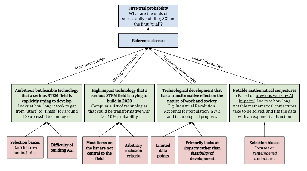
The first-trial probability asks, “what is the probability of successfully building AGI on the first ‘trial’?”. This is very hard to determine just on the surface, and so Davidson turns to several historical examples from a few reference classes. In particular, he looks at:
- ~10 examples of ambitious but feasible technologies that a serious STEM field is explicitly trying to develop (analogously, the field of AI is explicitly trying to achieve the ambitious but likely achievable goal of AGI)
- Technologies that serious STEM fields are trying to build in 2020, that plausibly seem like they could have a transformative impact on society
- Previous technologies that have had a transformative impact on the nature of work and society
- Notable mathematical conjectures and how long it took for them to be resolved (if indeed they were)
Davidson uses these reference classes to derive constraints on the first-trial probability – this can be done by obtaining a base rate of successful trials from the past examples. Most of these don’t succeed in the first trial6, so one approach he uses is to look at how many successes there are after \(X\) trials, then works backwards using Laplace’s rule. He ultimately settles on a best guess first-trial probability of 4%.
It’s worth noting that these reference classes and upward adjustments from the other trial definitions are the most important part of the framework, and the choice of these reference classes makes a really big difference to the final conclusions.
Number of virtual successes

The number of virtual successes changes how quickly we should update based on our observation of failed trials.7 We want the size of this update to be reasonable, so we don’t want this number to be too large or too small. Davidson ultimately settles on 1 virtual success for most of the report, based on a combination of pragmatism, the plausibility of the prior8, and the plausibility about the update size given new evidence.9
Different choices of the number of virtual successes matter less when the first-trial probability is lower, because making a big update (in proportion) from the prior distribution matters less in an absolute sense when the initial priors are already small.
Regime start time
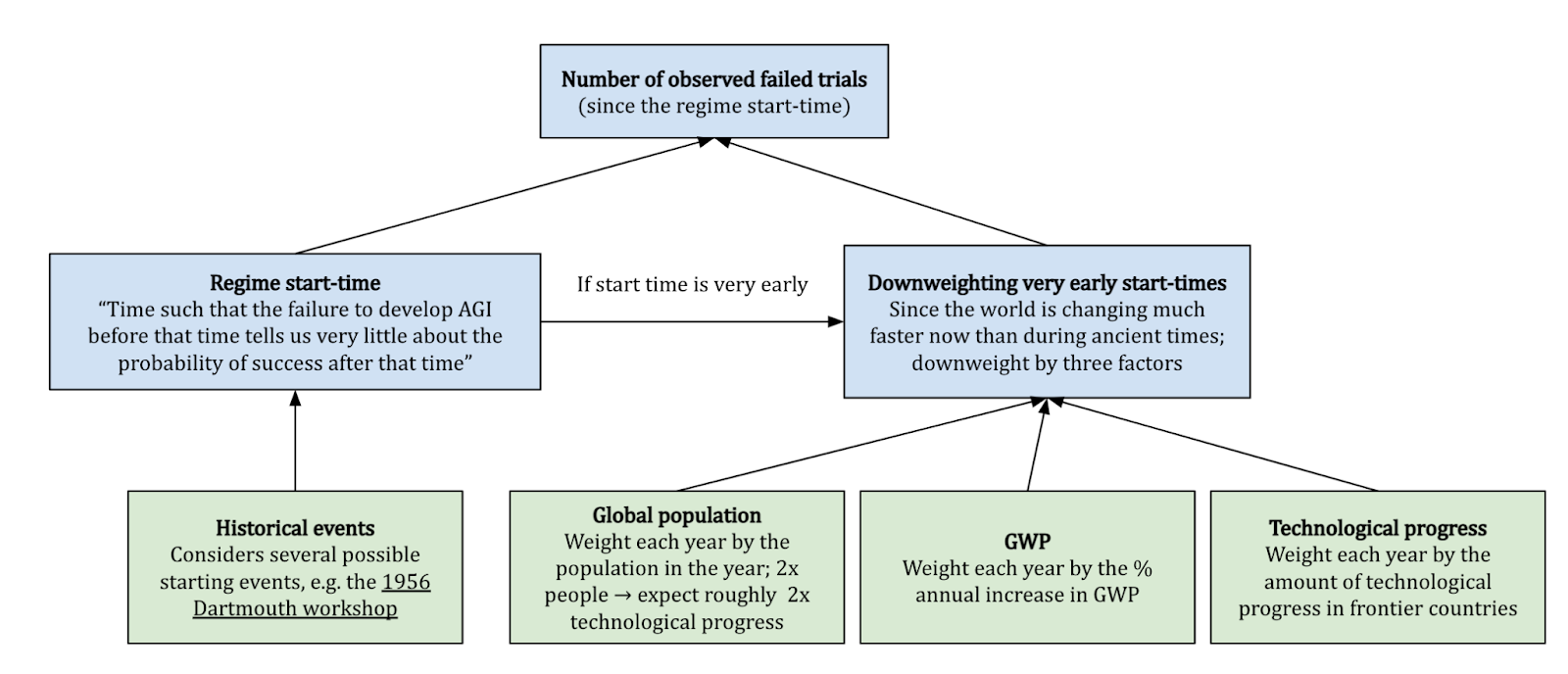
The regime start-time is the time for which “the failure to develop AGI before that time tells us very little about the probability of success after that time”, and affects the number of failed trials that we observe. While we previously considered the Dartmouth Conference in 1956 as the natural start of AI research, other alternatives (e.g. 1945, when the first digital computer was built) also seem reasonable.
A problem with assuming a constant probability \(p\) of AGI being developed in any year becomes especially salient if we consider very early start-times. Suppose we argue that people have been trying to automate parts of their work since ancient times, and choose a start-time correspondingly. Then the framework would suggest the odds of building AGI in any year in ancient times is the same as that today!
Davidson addresses this problem by down-weighting the number of trials occurring in ancient times relative to modern times, by multiplying (with normalisation!) each year by the global population or the economic growth in that year.10 Overall, he places the most emphasis on a start-time of 1956, but does a sensitivity analysis with several alternatives, which do not significantly change the conclusions when appropriate down-weighting is applied.
Trial definition
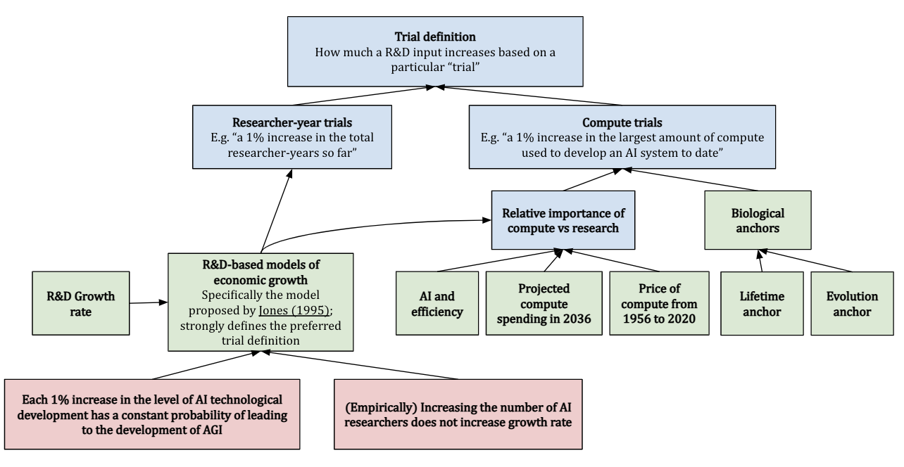
The final input to the framework is the trial definition, which specifies what exactly constitutes a single “trial” at building AGI. The initial approach we considered was in terms of calendar years, but there are reasonable alternatives, for example:
- Compute trials: Trials based on compute, e.g. 1 trial = “a 1% increase in the largest amount of compute used to develop an AI system to date”. These trials implicitly assume that increases in training compute are a key driver of AI progress11
- Researcher-year trials: Trials that are defined in terms of the number of researcher-years performed so far, e.g. 1 trial = “a 1% increase in the total researcher-years so far”. We’re in effect assuming that each 1% increase in the “level of AI technological development” has a constant probability of developing AGI.12
Davidson considers both of these possible trial definitions, together with the calendar-year definition, finding that the resulting probabilities can vary a little depending on the chosen trial definition. In effect, we now have three separate frameworks based on the trial definition:
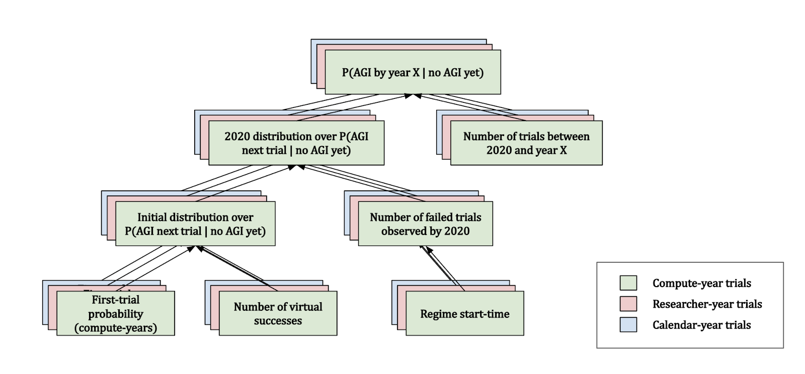
If we change the trial definition, then presumably we’ll also change the first-trial probability, so how do we calculate this? One approach that Davidson takes is to compute the first-trial probability for compute-years and researcher-years from the first-trial probability for calendar years – I’ll not go into this here, but I suggest looking at these sections of the report to find out more.
Assuming 1 virtual success and a regime start-time of 1956, here’s what we get:
P(AGI by 2036) | |||
Trial definition | Low-end | Central estimate | High-end |
Calendar-year | 1.5% | 4% | 9% |
Researcher-year | 2% | 8% | 15% |
Compute trial | 2% | 15% | 25% |
Table from Davidson, 2021
Importantly, we can choose our first-trial probability such that our predictions remain the same for trivial changes in the trial definition, helping solve one of the aforementioned problems with applying Laplace’s rule of succession.13 Overall, Davidson assigns ⅓ weight to each of the three trial definitions considered.
Putting things together: Final distribution
Model Extensions
The framework also considers three extensions to the stuff outlined above:
- Conjunctive model of AGI: It considers treating AGI development as the conjunction of multiple independent tasks
- Hyperpriors over update rules: Updating a prior over what weight to assign to different update rules, which are themselves determined by the four inputs14
- Allow some probability that AGI is impossible
For the most part, these extensions don’t have a particularly large effect on the final numbers and conclusions.
Final Distribution
If we combine everything from above then we end up with the following distribution and predicted numbers15:

P(TAI before 2030) | P(TAI before 2050) | P(TAI before 2100) |
~6% | ~11% | ~20% |
10% | 50% | 90% |
~2044 | >2100 | >2100 |
Davidson highlights three main strengths of his framework:
- It quantifies the size of the update to \(P(\text{AGI next year} \mid \text{no AGI yet})\) based on observed failures
- It highlights the significance of intuitive parameters, e.g. the first-trial probability, regime start-time, and the trial definition
- It’s arguably appropriate for expressing deep uncertainty about AGI timelines, e.g. by avoiding claims about “what fraction of the research we’ve completed towards AGI”
He also points out some main weaknesses of the framework:
- It incorporates limited kinds of evidence which could be really informative, e.g. how close we are to AGI
- Its near term predictions are too high, because current AI systems are not nearly as capable as AGI, and the framework doesn’t account for this evidence16
- It’s insensitive to small changes in the definition of AGI
- It assumes a constant chance of success in each trial (although the conjunctive model of AGI proposed in the extension relaxes this assumption)
There are also some situations where it doesn’t make sense to use this framework – for instance, when we know what “fraction of progress” we’ve made towards achieving a particular goal. This can be hard to quantify for AGI development, but it’s actually closely related to an approach that the Median group has previously attempted.
Conclusion
I think this model suggests that developing AGI within this century is at least plausible – we shouldn’t dismiss the possibility of developing AGI in the near term, and that the failure to develop AGI to date is not strong evidence for low \(P(\text{AGI by 2036})\).
I personally found the approach taken in this report really interesting, particularly in terms of the solutions Davidson proposes to the problems posed by the rule of succession. This seems possibly very valuable for other work on forecasting. I encourage you to look at the report’s blog post17, and to try making your own predictions using the framework.
You can play with the diagrams here, where the boxes link to the corresponding part of the report.
Notes
-
Green boxes correspond to inputs, red boxes are assumptions or limitations, and blue boxes are classed as “other”.
-
I’ve written a summary of the report, if you’re interested!
-
One way to think about this is as a distinction between “inside view” and “outside view” approaches (however see also this post). Cotra’s bioanchors report takes an inside view, roughly based on the assumption that training compute is the biggest bottleneck to building TAI, and quantifying how much we’ll need to be able to train a transformative model. Davidson’s semi-informative priors report instead specifies very little about how AI development works, leaning more heavily on reference classes from similar technologies and a general Bayesian framework.
-
This is a variation of the sunrise problem, which was the original problem that Pierre-Simon Laplace was trying to solve.
-
This is of a course a somewhat dubious assumption, and we’ll come back to this later on.
-
Indeed, looking only at the base rate of successful first trials alone would have a big problem of sparsity – there’s just not enough historical data!
-
We could also think about the number of virtual trials rather than virtual successes, but Davidson decides against this. Loosely speaking, if we use virtual trials, then it’s not as easy to separate out the effects of the first-trial probability and the effects from observed failed trials (more).
-
The prior is defined using a Beta distribution parameterised by (1) the number of virtual successes, and (2) the inverse of the first-trial probability. See here for more information.
-
The “plausibility of the prior” focuses on the shape of the Beta distribution, e.g. whether or not you should expect the probability density to be larger in the interval [0, 1/1000] or [1/1000, 2/1000]. On the other hand, the “plausibility of the update” looks at your expected probability of building AGI next year should change given the outcomes of newly observed trials. For example (borrowing from the report), “If you initially thought the annual chance of developing AGI was 1/100, 50 years of failure is not that surprising and it should not reduce your estimate down as low as 1/600”.
-
This approach also applies to researcher-years and compute years, and is described more here.
-
Incidentally, this is a claim that’s central to another of Open Philanthropy’s Worldview Investigations, Forecasting TAI with biological anchors, which I’ve discussed in another post.
-
Note that this doesn’t imply that there’s an infinite probability of developing AGI in the first researcher-year of effort, because it’s not true that we’re starting from the “zero” level of AI technological development. Essentially, the regime start-time is not about “when the level AI technological development started increasing” – see this footnote for more on discussion.
-
For example, we would like our prediction for \(P(\text{AGI within 10 years})\) to remain the same even if we use a trial definition of 1 month instead of 1 year. Although using a trial definition of 1 month would ordinarily lead to more total observed trials and thus more updating, this effect is cancelled out by choosing a different first-trial probability.
-
More concretely, suppose you think that several different updates rules (corresponding to e.g. different numbers of virtual successes) all seem reasonable, and you’re uncertain what to do. One approach is to weight the results for the different choices of update rules, and use these rules to update the forecasts based on evidence. But we might also be interested in updating how we weight the update rules, which is where the hyper prior comes in (more).
-
These numbers were extracted using WebPlotDigitizer.
-
Depending on your point of view, this may not be very compelling evidence – e.g. you might think that the ramp up to AGI would be extremely fast due to the discovery of a “secret sauce”.
-
You can also have a look at the full report if you want to get into the details!

