In last week’s Gradient Updates issue, I discussed how we can guess that GPT-4o and Claude 3.5 Sonnet have significantly fewer parameters than GPT-4. The most common question I’ve received from readers was some version of the following:

Don’t active parameters matter more for inference economics than total parameters? If so, how can you infer the total number of parameters of a model by only looking at its inference cost and speed?

In response to this, I’ve decided to make this issue specifically about the question of inference with mixture-of-experts (MoE) models. The basic takeaway is that MoEs are more efficient at inference than dense models of the same total parameter count, but less efficient than dense models with the same active parameter count. A rough rule of thumb is that an 8-way sparse model has the same short-context decoding economics as a dense model half its size.

For the sake of brevity, I’ll assume familiarity with basic concepts in Transformer inference, so I expect this issue to be confusing to readers without this necessary background. If you’re one of these readers, I recommend reading Pope et al’s paper on Transformer inference, kipply’s post on inference arithmetic, and Jacob Steinhardt’s post on how fast we can perform a forward pass before this post.

Gradient Updates

Weekly commentary on AI news and developments.

Advantages of MoE models

There are four main advantages of MoE models over dense models when it comes to inference, holding total parameter count fixed:

1. MoE models have fewer active parameters than dense models. This is the source of their advantage when we have the luxury of doing forward passes slowly.

2. MoEs tend to be shallower and wider than dense models.

3. MoEs tend to need less network communication per forward pass compared to a dense model of the same size and model depth.

4. MoEs tend to have smaller attention blocks, i.e. the product of their number of attention heads with the head dimension is smaller. This might make them cheaper to serve in long contexts, but whether this happens depends on whether we assume grouped-query or multi-query attention are used.

I’ll discuss each of these advantages in turn. Overall, (1) dominates when forward passes can be done slowly but becomes irrelevant when they must be done sufficiently fast. (2) and (3) are more significant when forward passes must be done quickly. (4) means MoEs are cheaper than similarly sized dense models in long-context inference.

MoEs have fewer active parameters than dense models

The most discussed advantage of MoE models over dense models is that we do less arithmetic (or FLOP) per token processed or generated, because only a small fraction of the parameters of our model will be active - in other words, be multiplied and accumulated - for each token. If arithmetic is the binding constraint on a forward pass, then using an MoE model instead of a dense model of the same size is going to lead to cheaper and faster inference because not all the parameters of the MoE will be active.

The key caveat in this is arithmetic has to be the binding constraint. In practice, this is only sometimes true.

In prefill, we have the advantage of processing all of the input tokens in parallel. Because of this, the single forward pass that processes all tokens in an input sequence at once can be quite slow: for example, it’s acceptable to spend 1 second to process an input sequence of 1000 tokens. Under these conditions, network latency is not an issue, and memory bandwidth is not a binding constraint because the batch size in units of processed tokens is large. Network communication can also be hidden behind arithmetic because the low network latency relative to the time taken for the forward pass allows more effective overlapping of communication with arithmetic as well as the use of higher bandwidth communication protocols. As a result of all of this, prefill costs are dominated by how much arithmetic needs to be done, and MoE models have a big advantage over dense models at fixed model size.

All of the above still remains true in decoding if we go slowly by using large batch sizes and small numbers of GPUs per instance. However, going faster requires increasing instance sizes to split arithmetic and memory workload over more GPUs, and this adds additional network communication overhead. To reduce the time taken by network communication, we need to scale down batch sizes beyond the critical batch size, i.e. the point where the time taken up by arithmetic and memory reads is equal. This means the memory reads for our matrix multiplications take longer than the arithmetic, and in this situation MoEs lose their active parameter advantage over dense models. The batch size at which this happens can be estimated by dividing the FLOP/s of a GPU by its memory bandwidth in units of TB/s. For the H100, it’s around 300.

To demonstrate how much time can be taken up by network communication at large batch sizes, consider serving Llama 3.3 70B for inference on a single node of H100s with 8-way tensor parallelism. In the feedforward blocks alone, each token processed will require 8192 words to be all-reduced for each layer, as 8192 is the model dimension. At an activation precision of 16 bits this amounts to 1 MB per token, and at the critical batch size of 300 we need to all-reduce 300 MB of data per forward pass. The low latency NVLink all-reduce protocol on the H100 offers an all-reduce bandwidth of 112 GB/s, so just the feedforward all-reduces alone take 2.7 milliseconds per token ignoring latency, compared to around 5 milliseconds this setup would need for the arithmetic. For context, 5 ms per token is about how fast Fireworks serves their version of Llama 3.3 70B. It’s not feasible to achieve such speeds at anywhere close to the critical batch size.

MoEs are shallower and wider than dense models

Though the smaller number of active parameters is the key advantage of MoEs over dense models, it’s not the only one. MoEs also tend to be shallower and wider than dense models at the same parameter count, and this gives them an advantage in inference economics because more serial computation is substantially harder to speed up than more parallel computation.

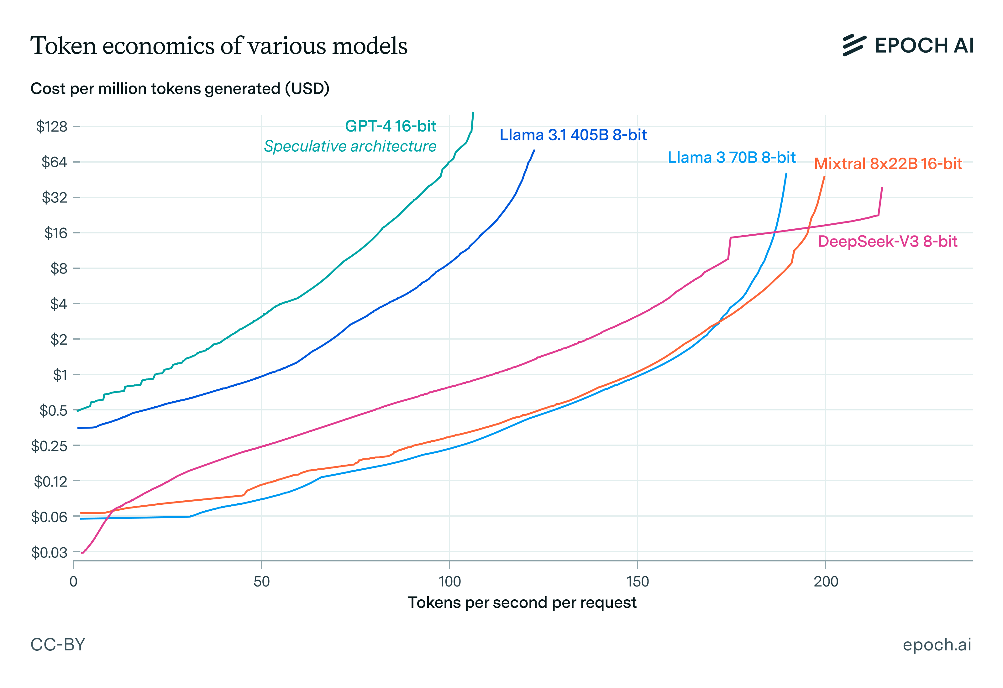
As an example of this general tendency, Mixtral 8x22B is a 140 billion parameter model with 56 layers, while Llama 3 70B is a 70 billion parameter model with 80 layers. This smaller number of layers is an advantage that matters most in fast short-context decoding, as in this case the number of layers of the model determines the number of times we’ll have to take network latency hits during the forward pass. Shallower and wider models also require less network communication, which is another advantage MoEs tend to have over similarly sized dense models.

If we assume MoE depth is scaled similarly to a dense model with the same number of active parameters, then we expect the inference economics of an MoE to be better than a dense model of the same overall size but worse than a dense model with the same number of active parameters. This is because both model depth and total parameter count matter for inference economics: the former determines how many times we take latency hits during a forward pass, and the latter determines how much information we need to read from HBM for generated tokens.

At fixed model depth, MoE models need less network communication than dense models

The amount of network communication for the feedforward blocks needed per processed or generated token scales with the product of the model dimension, the model depth, and the number of active experts if we hold batch size and the hardware setup fixed. Using this, we can compare MoE models to dense models of the same depth and parameter count in how much network communication they would require.

Let’s start with GPT-4. A dense model of the same depth and parameter count as GPT-4 would have to have a model dimension that’s 4 times greater, as parameter count per layer scales with the square of the model dimension and GPT-4 has 16 experts in total. Because GPT-4 has 2 active experts, we can see from the above product scaling that GPT-4 needs 50% less communication compared to a dense model of the same size and depth.

Generalizing this argument, we can see that as long as the number of active experts in an MoE is less than the square root of the overall number of experts, the MoE will have a network communication advantage over a dense model of the same total parameter count and model depth. This condition holds for GPT-4, and it also holds for models such as Mixtral 8x22B which have 8 total experts with 2 of them active.

In practice, MoEs tend to have an even bigger advantage over dense models than what I’ve calculated here because my calculation assumes model depth is held fixed. In practice, MoEs are also shallower and wider as covered earlier, and this increases their communication advantage further over dense models of the same size.

MoEs have smaller attention blocks than dense models

The attention blocks of MoE models are often sized according to what would be appropriate for a model consisting only of a single expert in the feedforward block. For example, GPT-4’s attention blocks are about the same size as GPT-3’s at 55 billion parameters total, even though GPT-4 is around 10 times bigger in total parameter count. Part of this is because GPT-4 uses multi-query attention, but this would only account for a 3x discrepancy. So GPT-4’s attention block is still around 3 times smaller than we would expect from a similarly sized dense model.

This discrepancy can make MoE models cheaper to inference in long contexts compared to dense models of the same size, because both the arithmetic cost and the KV cache read cost of attention scale with the product of the number of attention heads with the head dimension, assuming the attention group size for key and value heads is fixed. However, if instead we consider scaling up the attention group size proportionally to the number of attention heads, then the size of the KV cache per token remains fixed as we scale, so we get no benefit from the attention blocks becoming smaller.

In practice, the effect size we can expect here is quite small. Even in the most optimistic case for these savings, i.e. assuming grouped-query attention with a fixed group size, we only expect the KV cache size per token to scale with the cube root of the model size. So an MoE model with 16 experts would perhaps be 60% cheaper to inference than a dense model of the same size. This is much smaller than the effect of using grouped-query attention, which by itself reduces the size of the KV cache by a factor of 8 in Llama 3 70B and Llama 3 405B.

Estimating the MoE inference edge

Now, let’s try to get a quantitative estimate for the size of the MoE inference edge from all of the above considerations. As before, I’ll take GPT-4 as a reference model for simplicity, and I’ll assume that the depth and both dimensions of the weight matrices of a dense model each scale with the cube root of its size.

Given these, we can infer the following:

• The arithmetic cost of GPT-4 is equivalent to a dense model with 275B parameters.
• The memory bandwidth cost of GPT-4 is equivalent to a dense model with 1.8T parameters.
• The serial depth of GPT-4 is about as big as a model with 400B parameters (since it has 120 layers compared to the 126 layers of Llama 3 405B).
• The inter-GPU data movement cost of GPT-4 is half that of a dense model with 1.8T parameters and equivalent to a dense model with around 635B parameters under the above scaling assumptions.
• The attention block size of GPT-4 is equivalent to a dense model with 300B parameters, as it’s around 75% of the size of Llama 3 405B’s attention block.

For prefill or slow short-context decoding, GPT-4 essentially behaves like a dense model with 275B parameters. There’s nothing surprising here, as in this regime forward passes are arithmetic bound due to the large batch sizes and sequence lengths used. We get a cost saving equal to the sparsity factor of the model.

For fast short-context decoding, we know arithmetic cost is irrelevant as batch sizes tend to be too small in that regime. If we assume memory read time and network time (both latency and bandwidth) matter about the same, then a natural way to estimate a “dense model equivalent” size for GPT-4 is to weigh memory bandwidth cost by 0.5 and both serial depth and network communication by 0.25 in a geometric mean. This is because the last two factors together determine the total network communication time. Doing this, we obtain a “dense equivalent size” for fast short-context decoding of around 950B parameters for GPT-4.

In general, working through the calculation above in more detail suggests we should divide the total parameter count of an MoE by (number of experts)^(0.44) / (number of active experts)^(0.63) to get the dense equivalent size with the averaging we’ve chosen. For example, this suggests the 140 billion parameter Mixtral 8x22B should be equivalent to a dense model with around 90 billion parameters in fast short-context decoding.

In long contexts, the attention mechanism dominates cost, and it’s difficult to find a similar “dense equivalent size” because details such as the exact way in which KV heads are grouped together matter much more than the raw model size for inference economics.

Conclusion

Mixture-of-experts models are generally cheaper to serve for inference compared to dense models, but except in prefill this is not directly because they have a smaller number of active parameters. Instead, it’s because they tend to have fewer layers and need less network communication for a forward pass compared to dense models of the same size. So estimating the inference costs of an MoE by naively looking at its number of active parameters is going to be misleading.

If rough estimates of inference costs are needed, MoEs can be compared to dense models by computing a “dense equivalent model size” in the specific inference regime we’re considering. In fast short-context decoding, 4-way and 8-way sparse models are comparable to dense models with 65% and 50% of their total number of parameters respectively. Because of this, it’s probably easier to guess a model’s total parameter count compared to its active parameter count when you look at how fast the model is being served.