DeepSeek has recently released DeepSeek v3, which is currently state-of-the-art in benchmark performance among open-weight models, alongside a technical report describing in some detail the training of the model. Impressively, they’ve achieved this SOTA performance by only using 2.8 million H800 hours of training hardware time—equivalent to about 4e24 FLOP if we assume 40% MFU. This is about ten times less training compute than the similarly performing Llama 3.1 405B.
In this issue, I’ll cover some of the important architectural improvements that DeepSeek highlight in their report and why we should expect them to result in better performance compared to a vanilla Transformer. The full technical report contains plenty of non-architectural details as well, and I strongly recommend reading it if you want to get a better idea of the engineering problems that have to be solved when orchestrating a moderate-sized training run.

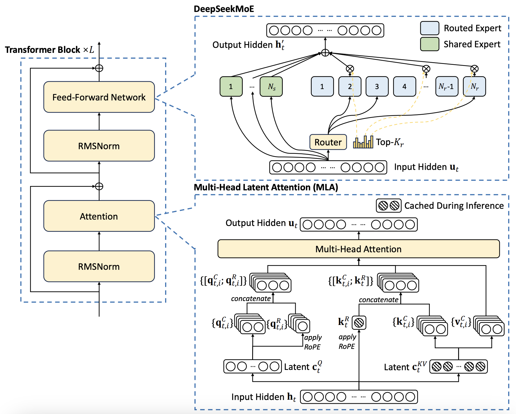
Figure 1: The DeepSeek v3 architecture with its two most important improvements: DeepSeekMoE and multi-head latent attention (MLA). Multi-token prediction is not shown. From the DeepSeek v3 technical report.
Multi-head latent attention (MLA)
Multi-head latent attention (abbreviated as MLA) is the most important architectural innovation in DeepSeek’s models for long-context inference. This technique was first introduced in DeepSeek v2 and is a superior way to reduce the size of the KV cache compared to traditional methods such as grouped-query and multi-query attention.
I’ll start with a brief explanation of what the KV cache is all about. If you’re familiar with this, you can skip directly to the next subsection.
What is the KV cache and why does it matter?
When a Transformer is used to generate tokens sequentially during inference, it needs to see the context of all of the past tokens when deciding which token to output next. The naive way to do this is to simply do a forward pass including all past tokens every time we want to generate a new token, but this is inefficient because those past tokens have already been processed before. We would just be recomputing results we’ve already obtained previously and discarded.
To avoid this recomputation, it’s efficient to cache the relevant internal state of the Transformer for all past tokens and then retrieve the results from this cache when we need them for future tokens. Because the only way past tokens have an influence on future tokens is through their key and value vectors in the attention mechanism, it suffices to cache these vectors. This is where the name key-value cache, or KV cache for short, comes from.
This works well when context lengths are short, but can start to become expensive when they become long. This is because cache reads are not free: we need to save all those vectors in GPU high-bandwidth memory (HBM) and then load them into the tensor cores when we need to involve them in a computation. If each token needs to know all of its past context, this means for each token we generate we must read the entire past KV cache from HBM.
In a vanilla Transformer using a standard multi-head attention mechanism, the number of KV cache parameters per past token can be expressed as:
2 * attention head dimension * number of attention heads * number of Transformer blocks
For instance, GPT-3 had 96 attention heads with 128 dimensions each and 96 blocks, so for each token we’d need a KV cache of 2.36M parameters, or 4.7 MB at a precision of 2 bytes per KV cache parameter.
GPT-3 didn’t support long context windows, but if for the moment we assume it did, then each additional token generated at a 100K context length would require 470 GB of memory reads, or around 140 ms of H100 time given the H100’s HBM bandwidth of 3.3 TB/s. The price per million tokens generated at $2 per hour per H100 would then be $80, around 5 times more expensive than Claude 3.5 Sonnet’s price to the customer (which is likely significantly above its cost to Anthropic itself). This naive cost can be brought down e.g. by speculative sampling, but it gives a decent ballpark estimate.
This rough calculation shows why it’s crucial to find ways to reduce the size of the KV cache when we’re working with context lengths of 100K or above. The most popular way in open-source models so far has been grouped-query attention. In this architectural setting, we assign multiple query heads to each pair of key and value heads, effectively grouping the query heads together - hence the name of the method. This cuts down the size of the KV cache by a factor equal to the group size we’ve chosen. In models such as Llama 3.3 70B and Mistral Large 2, grouped-query attention reduces the KV cache size by around an order of magnitude.
Beating grouped-query attention
The fundamental problem with methods such as grouped-query attention or KV cache quantization is that they involve compromising on model quality in order to reduce the size of the KV cache. Instead of this, DeepSeek has found a way to reduce the KV cache size without compromising on quality, at least in their internal experiments.
They accomplish this by turning the computation of key and value vectors from the residual stream into a two-step process. In a vanilla Transformer, key and value vectors are computed by directly multiplying the residual stream vector by a matrix of the shape
(number of heads · head dimension) x (model dimension)
DeepSeek’s method essentially forces this matrix to be low rank: they pick a latent dimension and express it as the product of two matrices, one with dimensions latent times model and another with dimensions (number of heads · head dimension) times latent. Then, during inference, we only cache the latent vectors and not the full keys and values. We can then shrink the size of the KV cache by making the latent dimension smaller.

Figure 2: An illustration of multi-head latent attention from the DeepSeek v2 technical report.
Naively, this shouldn’t fix our problem, because we would have to recompute the actual keys and values every time we need to generate a new token. After all, we need the full vectors for attention to work, not their latents. Multi-head latent attention is based on the clever observation that this is actually not true, because we can merge the matrix multiplications that would compute the upscaled key and value vectors from their latents with the query and post-attention projections, respectively.
The reason low-rank compression is so effective is because there’s plenty of information overlap between what different attention heads need to know about. If we used low-rank compression on the key and value vectors of individual heads instead of all keys and values of all heads stacked together, the method would simply be equivalent to using a smaller head dimension to begin with and we would get no gain. Exploiting the fact that different heads need access to the same information is essential for the mechanism of multi-head latent attention.
Methods such as grouped-query attention exploit the possibility of the same overlap, but they do so ineffectively by forcing attention heads that are grouped together to all respond similarly to queries. In other words, information sharing becomes coupled to having identical behavior in some restricted sense, a clearly undesirable property. Low-rank compression, on the other hand, allows the same information to be used in very different ways by different heads. In theory, this could even have beneficial regularizing effects on training, and DeepSeek reports finding such effects in their technical reports.
I see this as one of those innovations that look obvious in retrospect but that require a good understanding of what attention heads are actually doing to come up with. Once you see the approach, it’s immediately obvious that it cannot be any worse than grouped-query attention and it’s also likely to be significantly better. However, coming up with the idea of trying this is another matter.
Mixture-of-experts innovations
One of the most popular improvements to the vanilla Transformer was the introduction of mixture-of-experts (MoE) models. These models divide the feedforward blocks of a Transformer into multiple distinct experts and add a routing mechanism which sends each token to a small number of these experts in a context-dependent manner. This means the model can have more parameters than it activates for each specific token, in a sense decoupling how much the model knows from the arithmetic cost of processing individual tokens. Probably the most influential model that is currently known to be an MoE is the original GPT-4.
Expert routing algorithms work as follows: once we exit the attention block of any layer, we have a residual stream vector that is the output. Each expert has a corresponding expert vector of the same dimension, and we decide which experts will become activated by looking at which ones have the highest inner products with the current residual stream.
The problem with this is that it introduces a rather ill-behaved discontinuous function with a discrete image at the heart of the model, in sharp contrast to vanilla Transformers which implement continuous input-output relations. This causes gradient descent optimization methods to behave poorly in MoE training, often resulting in “routing collapse”, where the model gets stuck always activating the same few experts for every token instead of spreading its knowledge and computation around all of the available experts.
To get an intuition for routing collapse, consider attempting to train a model such as GPT-4 with 16 experts in total and 2 experts active per token. Now, suppose that for random initialization reasons two of these experts just happen to be the best performing ones at the start. Gradient descent will then reinforce the tendency to pick these experts. This will mean these experts will get almost all of the gradient signals during updates and become better while other experts lag behind, and so the other experts will continue not being picked, producing a positive feedback loop that results in other experts never getting chosen or trained.
The fundamental issue is that gradient descent just heads in the direction that’s locally best. This usually works fine in the very high dimensional optimization problems encountered in neural network training. However, when our neural network is so discontinuous in its behavior, even the high dimensionality of the problem space may not save us from failure.
It is nontrivial to address these training difficulties. DeepSeek v3 does so by combining several different innovations, each of which I will discuss in turn.
Auxiliary-loss-free load balancing
A popular method for avoiding routing collapse is to force “balanced routing”, i.e. the property that each expert is activated roughly an equal number of times over a sufficiently large batch, by adding to the training loss a term measuring how imbalanced the expert routing was in a particular batch. This term is called an “auxiliary loss” and it makes intuitive sense that introducing it pushes the model towards balanced routing. However, the DeepSeek v3 technical report notes that such an auxiliary loss hurts model performance even if it ensures balanced routing.
Their alternative is to add expert-specific bias terms to the routing mechanism which get added to the expert affinities. These bias terms are not updated through gradient descent but are instead adjusted throughout training to ensure load balance: if a particular expert is not getting as many hits as we think it should, then we can slightly bump up its bias term by a fixed small amount every gradient step until it does. The technical report notes this achieves better performance than relying on an auxiliary loss while still ensuring appropriate load balance.
Shared experts
A serious problem with the above method of addressing routing collapse is that it assumes, without any justification, that an optimally trained MoE would have balanced routing. However, this is a dubious assumption.
To see why, consider that any large language model likely has a small amount of information that it uses a lot, while it has a lot of information that it uses rather infrequently. For instance, almost any English request made to an LLM requires the model to know how to speak English, but almost no request made to an LLM would require it to know who the King of France was in the year 1510. So it’s quite plausible the optimal MoE should have a few experts which are accessed a lot and store “common information”, while having others which are accessed sparsely and store “specialized information”.
If we force balanced routing, we lose the ability to implement such a routing setup and have to redundantly duplicate information across different experts. However, if we don’t force balanced routing, we face the risk of routing collapse. To escape this dilemma, DeepSeek separates experts into two types: shared experts and routed experts. Shared experts are always routed to no matter what: they are excluded from both expert affinity calculations and any possible routing imbalance loss term. We concern ourselves with ensuring balanced routing only for routed experts.
The key observation here is that “routing collapse” is an extreme situation where the likelihood of each individual expert being chosen is either 1 or 0. Naive load balancing addresses this by trying to push the distribution to be uniform, i.e. every expert should have the same chance of being selected. However, if our sole concern is to avoid routing collapse then there’s no reason for us to target specifically a uniform distribution. DeepSeek v3 instead targets a distribution where each expert is either selected for sure (probability 1) or selected with some fixed probability p > 0 for each token.
I think it’s likely even this distribution is not optimal and a better choice of distribution will yield better MoE models, but it’s already a significant improvement over just forcing a uniform distribution.
Multi-token prediction
The final change that DeepSeek v3 makes to the vanilla Transformer is the ability to predict multiple tokens out for each forward pass of the model. This allows them to use a multi-token prediction objective during training instead of strict next-token prediction, and they demonstrate a performance improvement from this change in ablation experiments.
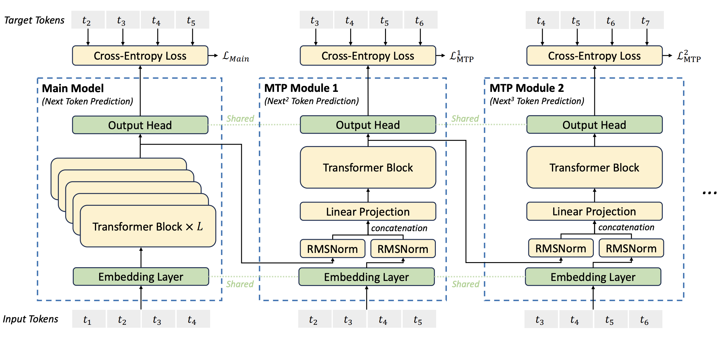
The basic idea is the following: we first do an ordinary forward pass for next-token prediction. As we would in a vanilla Transformer, we use the final residual stream vector to generate next token probabilities through unembedding and softmax. However, unlike in a vanilla Transformer, we also feed this vector into a subsequent Transformer block, and we use the output of that block to make predictions about the second next token. We can iterate this as much as we like, though DeepSeek v3 only predicts two tokens out during training.

Figure 3: An illustration of DeepSeek v3’s multi-token prediction setup taken from its technical report.
They incorporate these predictions about further out tokens into the training objective by adding an additional cross-entropy term to the training loss with a weight that can be tuned up or down as a hyperparameter. This not only gives them an additional target to get signal from during training but also allows the model to be used to speculatively decode itself. We can generate a few tokens in each forward pass and then show them to the model to decide from which point we need to reject the proposed continuation.
DeepSeek v3 only uses multi-token prediction up to the second next token, and the acceptance rate the technical report quotes for second token prediction is between 85% and 90%. This is quite impressive and should allow nearly double the inference speed (in units of tokens per second per user) at a fixed price per token if we use the aforementioned speculative decoding setup. It doesn’t look worse than the acceptance probabilities one would get when decoding Llama 3 405B with Llama 3 70B, and might even be better.
I’m curious what they would have obtained had they predicted further out than the second next token. If e.g. each subsequent token gives us a 15% relative reduction in acceptance, it might be possible to squeeze out some more gain from this speculative decoding setup by predicting a few more tokens out.
Conclusion
I see many of the improvements made by DeepSeek as “obvious in retrospect”: they are the kind of innovations that, had someone asked me in advance about them, I would have said were good ideas. However, as I’ve said earlier, this doesn’t mean it’s easy to come up with the ideas in the first place.
I’ve heard many people express the sentiment that the DeepSeek team has “good taste” in research. Based just on these architectural improvements I think that assessment is right. None of these improvements seem like they were found as a result of some brute-force search through possible ideas. Instead, they look like they were carefully devised by researchers who understood how a Transformer works and how its various architectural deficiencies can be addressed.
If I had to guess where similar improvements are likely to be found next, probably prioritization of compute would be a good bet. Right now, a Transformer spends the same amount of compute per token regardless of which token it’s processing or predicting. This seems intuitively inefficient: the model should think more if it’s making a harder prediction and less if it’s making an easier one. To some extent this can be incorporated into an inference setup through variable test-time compute scaling, but I think there should also be a way to incorporate it into the architecture of the base models directly.
About the authors


