Recently, we published the results of our investigation into data movement bottlenecks in distributed training of deep learning models, introducing a detailed model of the bandwidth and latency costs of different modes of parallelism in GPU clusters. Today, we’re also releasing an interactive simulator with a user-friendly interface implementing the same model.
This post will introduce the simulation tool’s features by using it to answer the following question: how big of a neural network training run could we have done using the GTX 580 GPUs that were used to train AlexNet in 2012? In other words, instead of training AlexNet on two GTX 580 3GB GPUs for six days, how far could an AI lab have scaled training if they wanted to train the largest possible model using just GTX 580 3GB GPUs, disregarding cost considerations?
How to use the tool
Before getting into the specific experiment to answer this question, let’s see how to get started with using the tool. On launch, you’ll be greeted with the following interface:

Figure 1: The user interface as it would be seen upon first launching the tool.
The plot of training FLOP versus model FLOP utilization is the primary output of the model: what utilization could we get if we performed a distributed training run as efficiently as possible at a particular training compute scale? The different tabs contain additional information about the optimal ways of scaling different dimensions of parallelism as training compute is increased and the maximum training compute that’s feasible to spend on training if we want our utilization to not fall below e.g. 80% of the maximum achievable sustained utilization on a particular GPU.
Above the upper right corner of the plot, a download button is available which you can use to obtain the complete output of our model beyond the summary information we display in the user interface. This output is structured as a JSON file and should be easy to parse using standard libraries.
The settings tab can be used to switch between different presets that correspond to the different plots from the paper. Each of these presets is a list of configurations, and each configuration consists of the following:
-
Scaling laws for important quantities such as training dataset size, critical batch size, model depth and model sparsity factor.
-
The GPU specification that’s to be used for the training runs in the configuration.
-
Assumptions about parallelism and communication: which scheduling scheme is used for pipeline parallelism, which kinds of network communication can be overlapped with computation, etc.
We model communication between GPUs in a hierarchical manner. There are increasingly large groups of GPUs that are connected to one another using increasingly slower interconnect. For example, one machine (or node) can host up to 8 H100 GPUs that can all talk to each other at 900 GB/s over NVLink, but the per-GPU bandwidth available for communication between different machines goes down to the InfiniBand bandwidth of 100 GB/s.
Overall, our tool requires the following information about the network setup:
-
How many levels of hierarchy are there in the network? This would be 2 if we model intra-node and inter-node communication, which is what we do by default; and would go up to 3 if we also model inter-datacenter communication.
-
For each level of hierarchy, what’s the per-GPU bandwidth available for communication at that level, counting both reads and writes? If in one second one GPU sends one byte to another GPU, this is counted as 2 bytes/second of communication. We adopt this convention to match NVIDIA’s NVLink bandwidth reporting.
-
For each level of hierarchy, what’s the latency of point-to-point communication at that level?
The user can also create their own custom configurations by clicking the “add new configuration” button and changing all of the settings from their default values. Upon clicking the “run simulation” button on the bottom right, the user’s new configuration will also be included in the plots displayed on the left-hand side. It’s also possible to include or exclude various configurations from any particular simulation run.
What would have been the largest feasible training run in 2012?
In 2012, Krizhevsky, Sutskever, and Hinton achieved breakthrough results on ImageNet using a deep convolutional neural network trained on two NVIDIA GTX 580 GPUs. Their model, which became known as AlexNet, took 5-6 days to train on 1.2 million images and demonstrated significantly better performance than previous approaches. The authors suggested their results could be improved simply by waiting for faster GPUs and bigger datasets.
This raises an interesting counterfactual question: what if the AlexNet team had access to a much larger compute budget in 2012? Instead of using just two GTX 580s, what if they had attempted to orchestrate the largest possible training run using the hardware available at that time? Our distributed training tool enables us to analyze this scenario by modeling the theoretical limits of scaling neural network training on GTX 580 hardware.
We’ll use this custom configuration function to perform our experiment with GTX 580 GPUs, which were state-of-the-art NVIDIA hardware in 2012. Here is a brief summary of their relevant specifications:
Table 1: Specs for the GTX 580 3GB GPU according to various sources. Most of these are taken directly from the GPU datasheet, but a few (such as network and matrix multiplication latency) are our guesses at what the real values might have been. These guesses are marked with the “speculative” tag.
| Category | Specification |
|---|---|
| Bitwidth (32) | 32 |
| FLOP/s (32) | 1.581e+12 (1.581 TFLOPS) |
| FLOP per clock per thread (32)1 | 1/2 |
| Bitwidth (64) | 64 |
| FLOP/s (64) | 197.6e+9 (197.6 GFLOPS) |
| FLOP per clock per thread (64) | 1/16 |
| Register bytes per processing block | 128 KiB |
| Number of streaming multiprocessors | 16 |
| L2 Bandwidth | 384.8e+9 Bps |
| L2 Bytes | 786,432 Bytes |
| Global Bandwidth | 192.4e+9 Bps |
| Maximum clock frequency | 1.544e+9 Hz (1.544 GHz) |
| Effective utilization | 85% (speculative) |
| High-bandwidth memory | 3.0e+9 Bytes (3 GB) |
| Latency per matrix multiplication | 2.25e-5 seconds (speculative) |
| Number of levels | 2 |
| Network bandwidth per level | Level 1: 8e+9 Bps Level 2: 1e+9 Bps |
| Network latency per level | Level 1: 5e-6 seconds (speculative) Level 2: 5e-6 seconds (speculative) |
| Level sizes | Level 1: 8 |
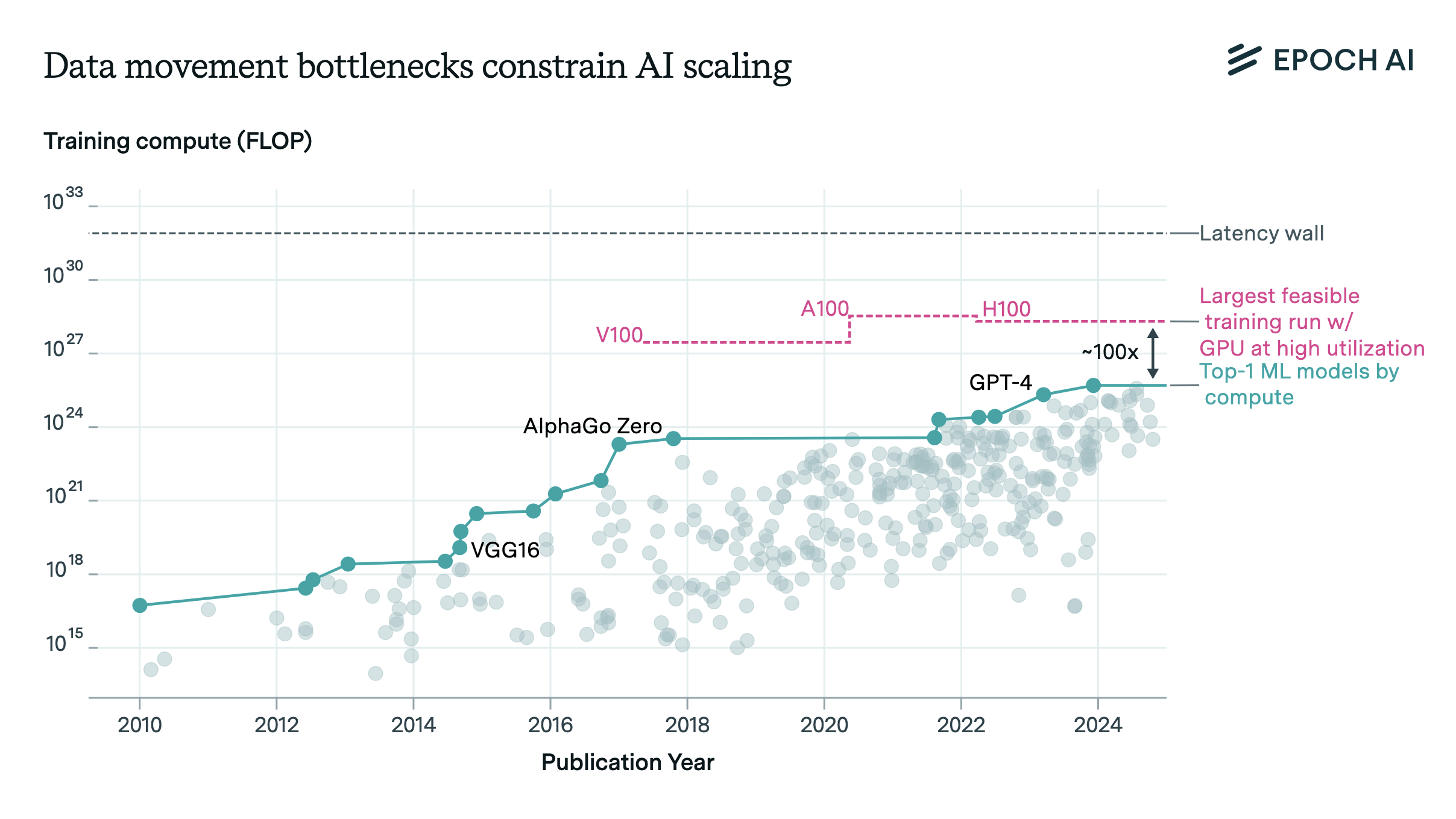
Plugging the specs of the GTX 580 3GB GPU into our tool, we find that the largest training run that could have been orchestrated using the GPUs used to train AlexNet over 3 months while remaining over 80% of peak utilization is 1e26 FLOP. In other words, the technology of the year 2012 was already enough to train a model as big as GPT-4 in 3 months, though this would have required 16 million GPUs in total. For a price of around $300 per GPU, the total cost of the GPUs alone would have been around $5 billion.2
We might also want to know how this 1e26 FLOP training run would be parallelized. The tool also allows us to answer this question: the optimal strategy for the feedforward block is 1024-way data parallelism, 32-way pipeline parallelism and 512-way tensor parallelism. It’s common practice today in frontier model training to use only tensor parallelism inside a single node of 8 GPUs, and our tool also confirms that this is the most efficient setup.
Figure 2: Results of the experiment with the GTX 580 3 GB GPU, shown together with the V100, A100 and H100 utilization curves for comparison.
Our interactive tool is not limited to historical scenarios—it can also help answer a wide range of questions about frontier ML model training at scale. For example, you might explore the largest feasible training runs with today’s cutting-edge hardware, or investigate how future improvements in network latency and bandwidth could expand these limits. By adjusting hardware specifications and communication assumptions within the tool, you can simulate how different factors impact training efficiency and scalability.
Finally, if you’re interested in how the tool works behind the scenes, you can find the model that it’s based on in this repository.
Notes
-
This particular data point can be confusing because our GPU model assumes operations are being done on tensor cores with 32 threads per tensor core and 4 tensor cores per streaming multiprocessor. The GTX 580 doesn’t use tensor cores, but we can still pick the value here such that (clock frequency) * (128 threads per SM) * (16 SMs) * (FLOP per clock per thread) is equal to 1.581e12 FLOP/s, which is reported in the GPU datasheet.
-
The actual budget it took to purchase the GPUs in the cluster GPT-4 was trained on was around $400 million: around 20,000 A100s at a price of $20,000 per GPU.
About the authors


